TODAY: Neural Networks - IV
- Convolutional neural network
- Recurrent neural network
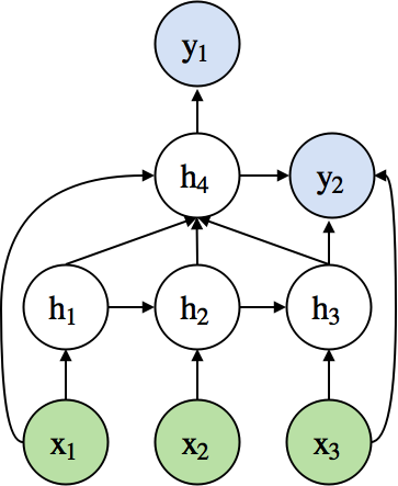
FAQ: Does a neural network have to be always layer-structured?
- No. It can be any directed acyclic graph (DAG).
- Example of a complex neural network
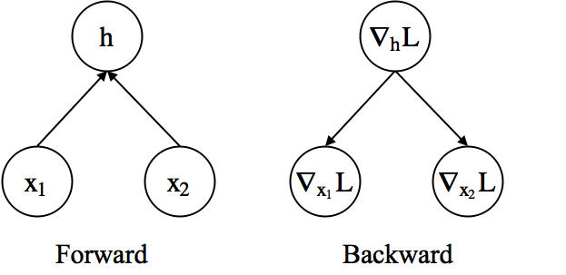
FAQ: Can we define any arbitrary layers?
- We can define any layer as long as it is differentiable.
- When it is not differentiable, we can make it approximately so.
- Example) Addition layer
- Forward: $\textbf{h} = \textbf{x}_1 + \textbf{x}_2$
- Backward
- $\nabla_{\textbf{x}_1}\mathcal{L} = \nabla_{\textbf{h}}\mathcal{L}\nabla_{\textbf{x}_1}\textbf{h}=\nabla_{\textbf{h}}\mathcal{L}$
- $\nabla_{\textbf{x}_2}\mathcal{L} = \nabla_{\textbf{h}}\mathcal{L}\nabla_{\textbf{x}_2}\textbf{h}=\nabla_{\textbf{h}}\mathcal{L}$
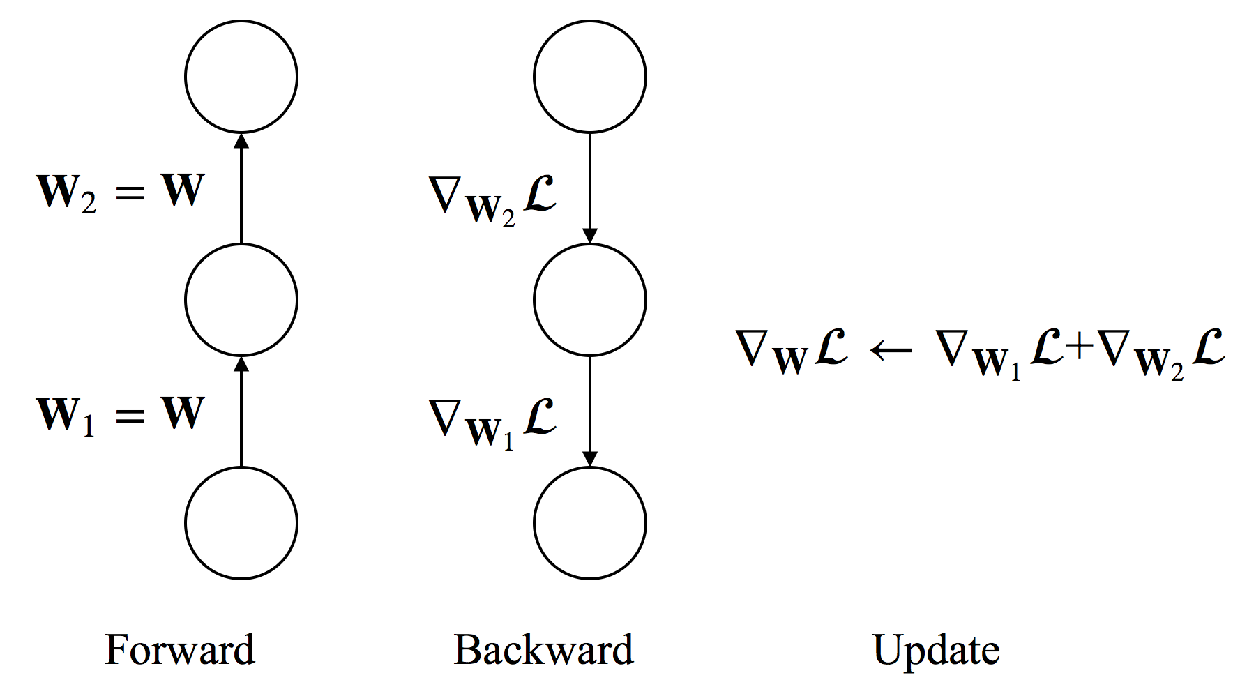
FAQ: How to handle shared weights?
- To constrain $W_1=W_2=W$, we need $\Delta W_1 = \Delta W_2$.
- Compute $\nabla_{W_1}\mathcal{L}$ and $\nabla_{W_2}\mathcal{L}$ separately.
- Use $\nabla_{W}\mathcal{L}=\nabla_{W_1}\mathcal{L}+\nabla_{W_2}\mathcal{L}$ to update the shared weight.
- In practice, we accumulate gradients to the shared memory space for $\nabla_{W}\mathcal{L}$ during back-propagation.
- Weight sharing is used in convolutional neural networks and recurrent neural networks.
What is "deep" neural network?
- If we have to given a definition...
- A neural network is considered to be deep if it has more than two (non-linear) hidden layers.
- Higher layers extract more abstract and hierarchical features.
- Difficulties in training deep neural networks
- Easily overfit (The number of parameters is large)
- Hard to optimize (highly non-convex optimization)
- Computationally expensive (many matrix multiplications)
- Recent Advances
- Large-scale dataset (e.g., 1M images in ImageNet)
- Better regularization (e.g., Dropout)
- Better optimization (e.g., Adam family)
- Better hardware (GPU/TPU for matrix computation)
Popular Deep Architectures
- Convolutional Neural Network (CNN)
- Widely used for image modeling
- e.g. object recognition, segmentation, vision-based reinforcement learning problems
- e.g. flow analysis and modeling (i.e. thinking the flow field as 2D/3D images)
- Recurrent Neural Network (RNN)
- Widely used for sequential data modeling
- e.g. machine translation, image caption generation
- e.g. time series analysis and forecasting, nonlinear dynamics
Convolutional Neural Network
- A special kind of multi-layer neural network
- Traditionally designed to recognize visual patterns directly from raw pixels
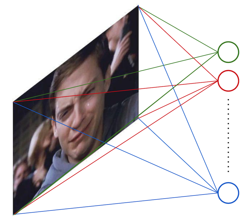
Multi-layer Perceptron (MLP)
- Consider 100x100 input pixels
- 1 hidden layer with 10000 hidden units
- 100M parameters $\rightarrow$ infeasible!
$\rightarrow$ Pixels are locally correlated!
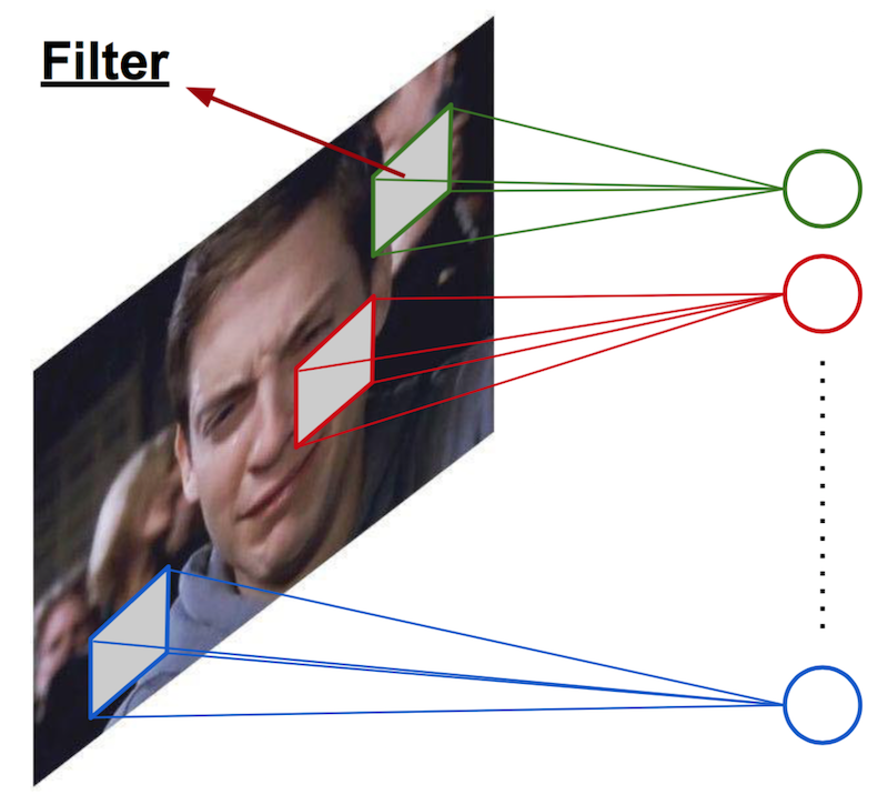
Locally-connected Neural Network
- Consider 100x100 input pixels
- Each unit is connected to 10x10 pixels.
- Each unit extracts a local pattern from the image.
- 10000 hidden units
- 1M parameters $\rightarrow$ still too large
Convolutional Neural Network (one filter)
- Consider 100x100 input pixels
- Apply the same filter (weight) over the entire image.
- Hidden units form a 100x100 feature map.
- 10x10 parameters.
$\rightarrow$ only captures a single local pattern.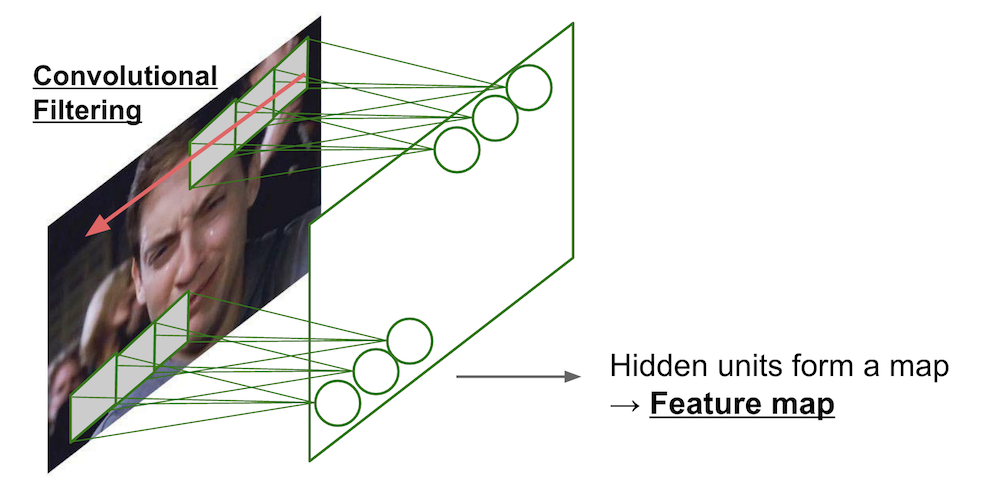
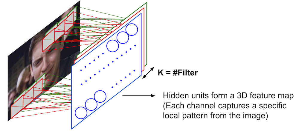
Convolutional Neural Network (multiple filters)
- 100x100 input pixels
- Apply K number of 10x10 filters.
- Hidden units form a Kx100x100 feature map.
- Kx10x10 parameters.
- Num of filters and size of filters are hyperparameters.
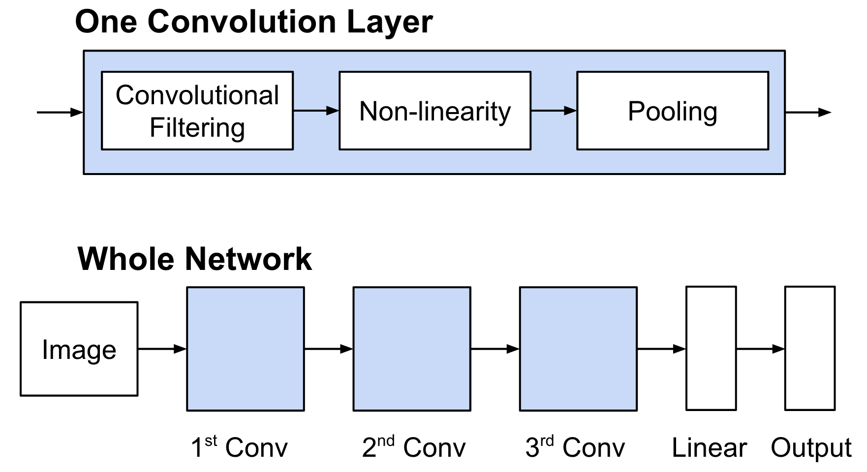
Typical Deep CNN Architecture
Details of Convolution
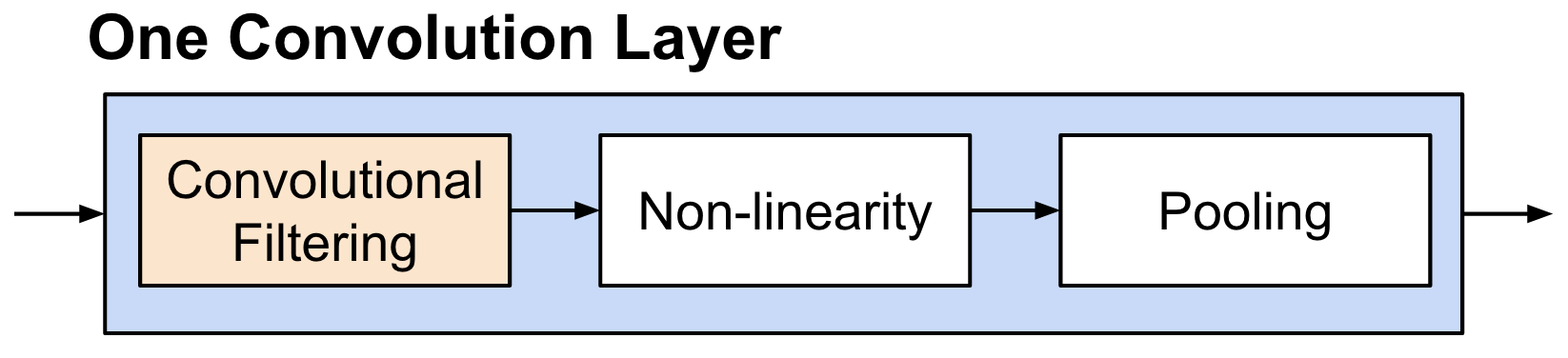
Details of Convolution: Convolutional Filtering
- A filter has $\textbf{W} \in \mathbb{R}^{h \times w}$ weights (bias is omitted for simplicity).
- Compute inner products between $\textbf{W}$ and $h \times w$ input patches by sliding window.
- The same weight is shared across the entire image.
- The following animation shows the simplest case: one-channel input, one filter
 (Figure from Stanford UFLDL Tutorial)
Details of Convolution: Convolutional Filtering
- In general, an input consists of multiple channels.
- Each filter has $\textbf{W} \in \mathbb{R}^{c \times h \times w}$ weight ($c$: #channels of input).
- Applying $K$ different filters $\rightarrow$ produces a 3D feature map (stacked through channels).
- Hyperparameters: num of filters, size of filters
- The following figure shows the general case: multi-channel input, mutilple filters
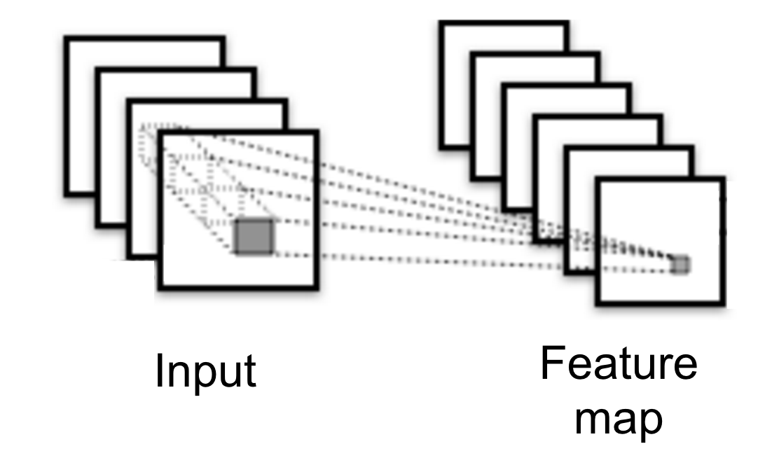 (Figure from Yann LeCun)
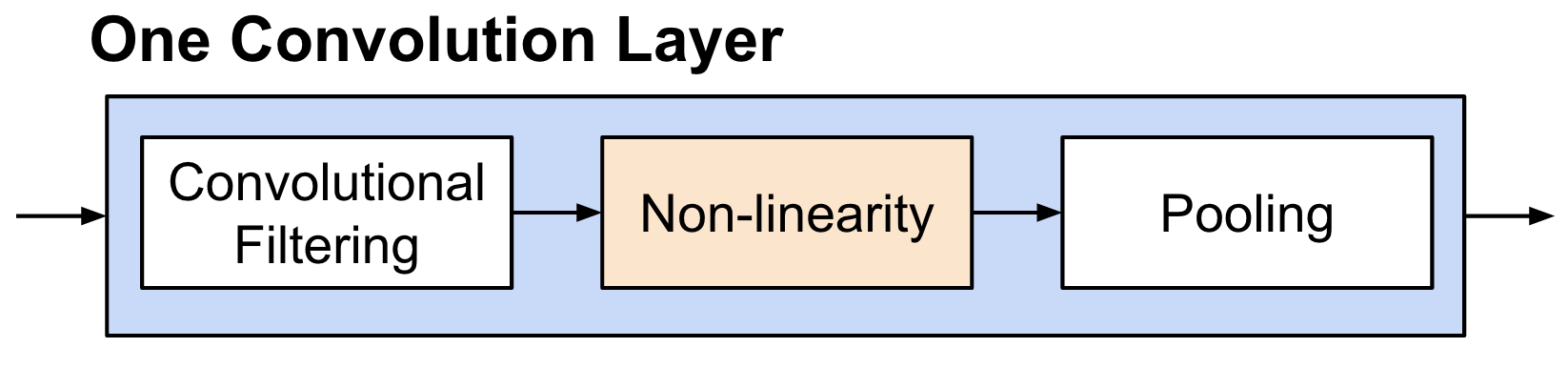
Details of Convolution: Non-linearity
- Method: Just apply non-linear function (e.g., Sigmoid, ReLU)
- ReLU is preferred because it is easier to optimize.
Details of Convolution: Pooling
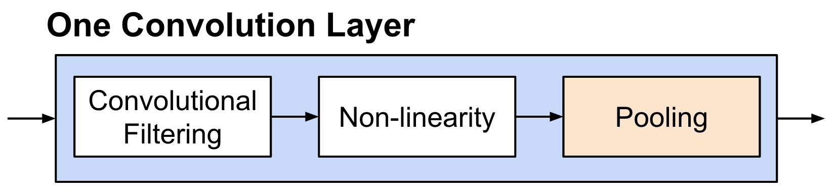
Details of Convolution: Pooling
- Method: Take average or maximum over HxW region of input feature.
- Outcome
- Shrink the number of hidden units.$\rightarrow$ reduces the number of parameters at the end.
- Make features robust to small translations of image.
- Hyperparameters: pooling method (avg or max), pooling size
- Often called "sub-sampling"
 (Figure from Stanford UFLDL Tutorial)
Illustration of Deep CNN
- Feature maps become smaller in higher layers due to pooling.
- Hidden units in higher layers capture patterns from larger input patches.
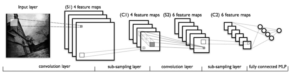 (Figure from Yann LeCun)
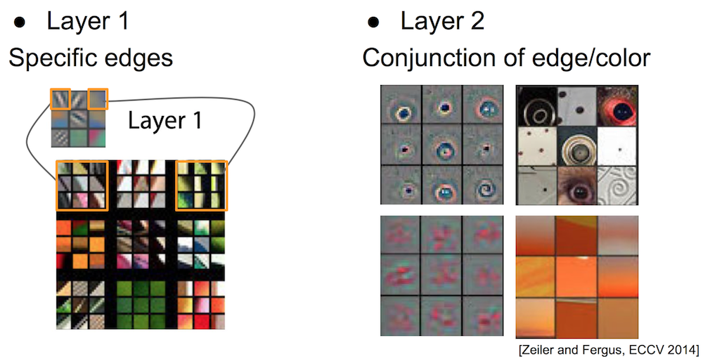
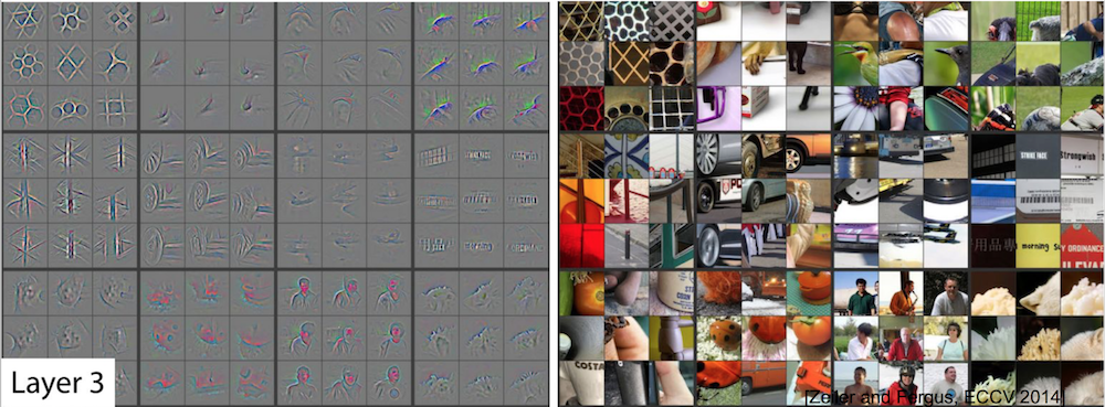
What is learned by CNN? Filter Visualization
- Train a deep CNN on ImageNet (1.2M images, 1000 classes)
- Perform forward propagations from many examples
- Find image patches that strongly activate a specific feature map (filter)
- Reconstruct the input patch from the feature map
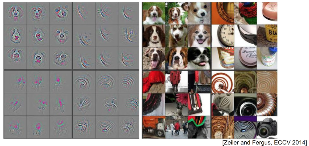
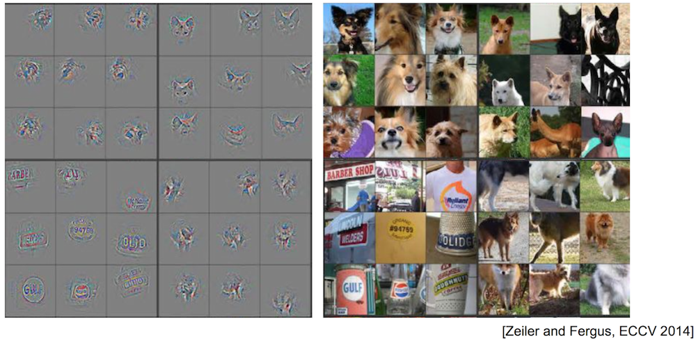
- Proposed by Zeiler and Fergus (ECCV 2014)
Filter Visualization: 1st and 2nd Layer
Filter Visualization: 3rd Layer
- Shows more complex patterns
Filter Visualization: 4th Layer
- More class-specific
Filter Visualization: 5th Layer
- Shows entire objects with pose variations
- Each filter can be viewed as a part detector. (e.g., dog face, text, animal leg)
An online interactive CNN visualization example:
Comparison to Traditional Approach
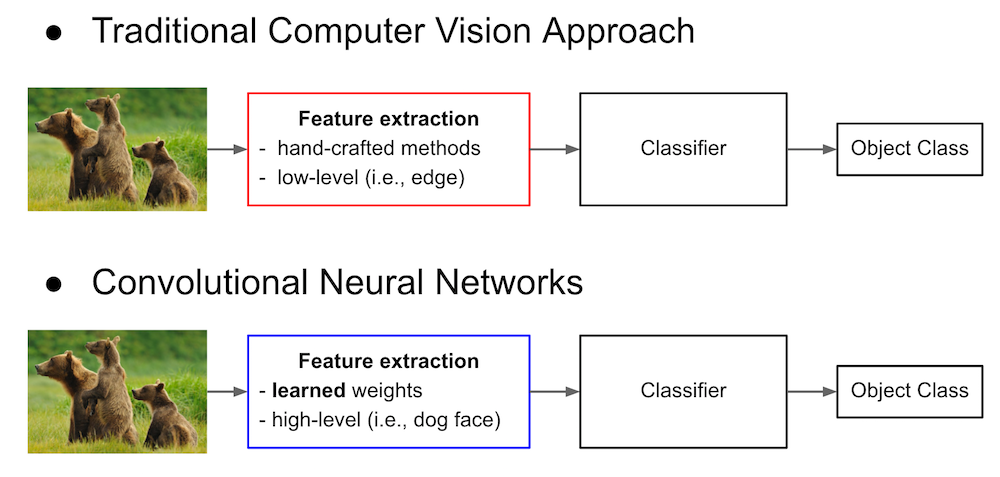
Summary of Convolutional Neural Network
- Convolutional Neural Network: a special kind of neural network with local connectivity and weight sharing.
- Achieves state-of-the-art performances on many different computer visoin tasks.
- Higher layers extract high-level features (e.g., dog face).
- Learned features can be generally used for other vision tasks.
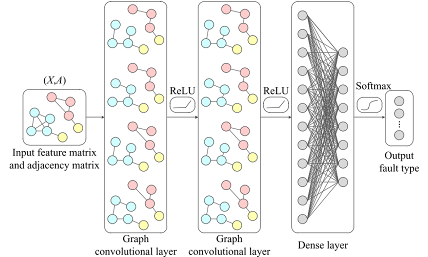
Graph Convolutional Network
But not all data reside in a regular array-like space. In particular, networks
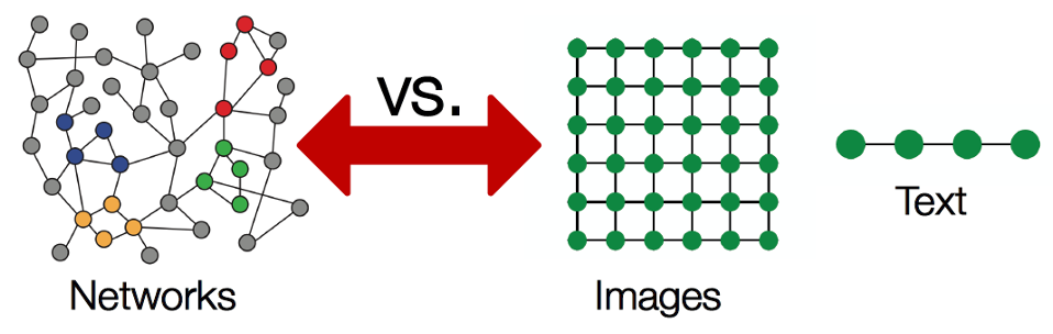
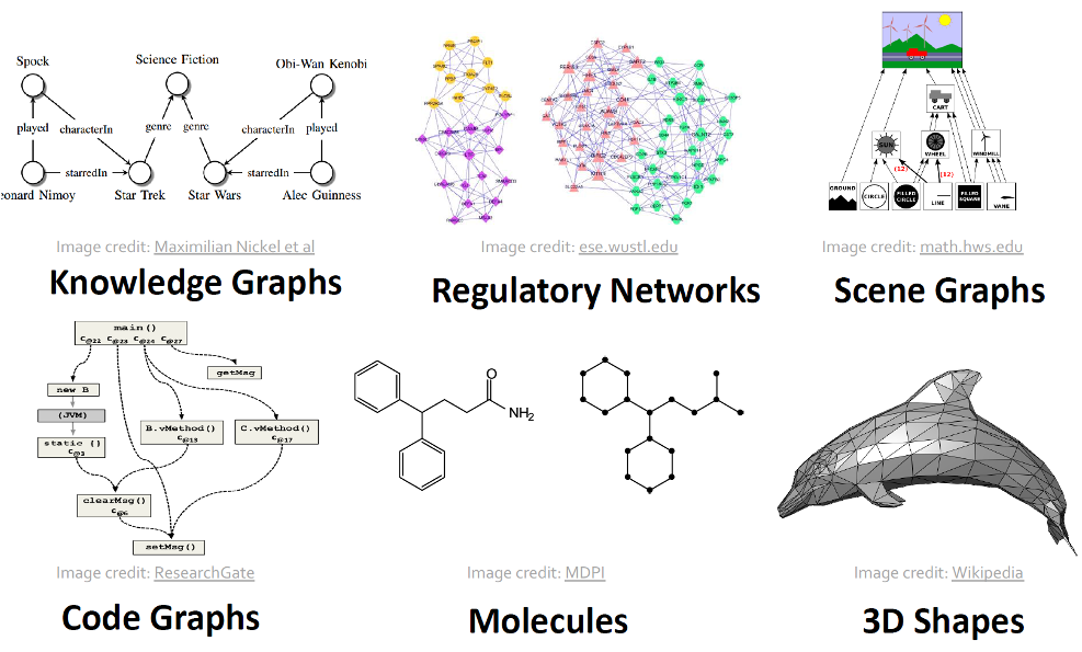
Examples of networks, or graph-based data structure
Convolution on array viewed as graph
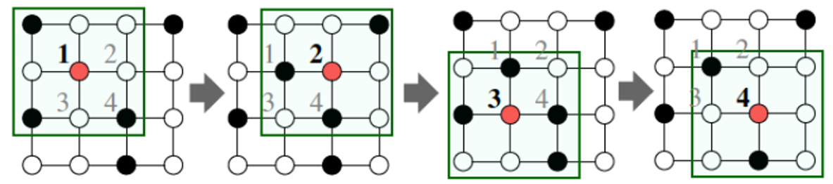
Convolution on Graph
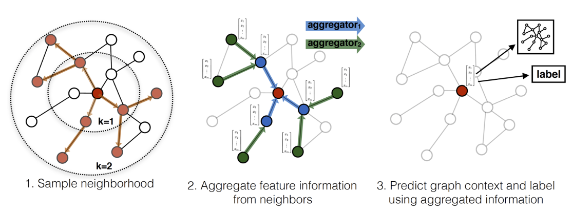
Message Passing Mechanism
Generalized convolution
- Consider a node $v$ and its neighbors $\cN(v)$, all having a feature vector $\vh$
- Aggregation: Gather information $\vh_u^{(j)}$ from neighbors $u\in\cN(v)$
- Update: Compute new features $\vh_v^{(j+1)}$ from the gathered information $\vm^{(j)}$
Example GNN
Example Application in Fluid Dynamics - Ship Airwake
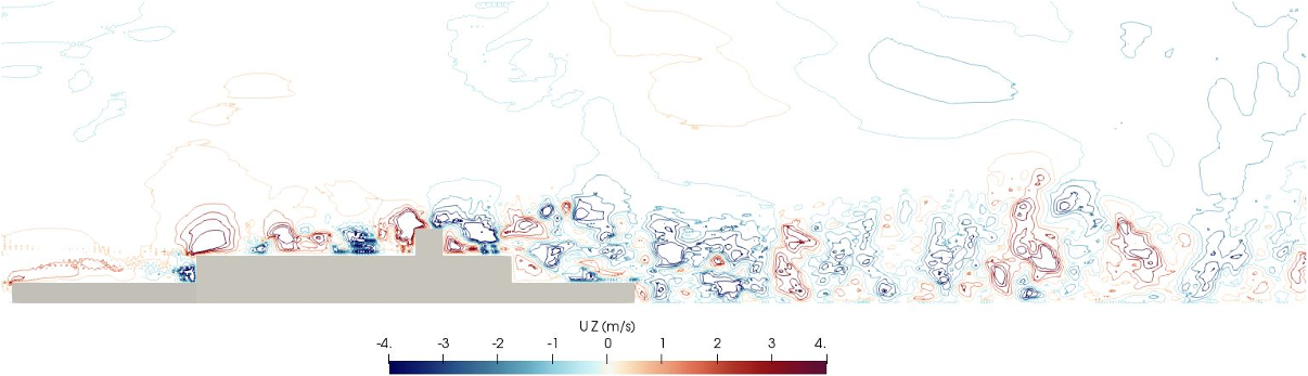
Example Application in Fluid Dynamics - Vortical Dynamics in Airwake
Recurrent Neural Networks (RNN)
- A special kind of neural network designed for modeling sequential data
- Can take arbitrary number of inputs
- Can produce arbitrary number of outputs
- Examples of sequential problems
- Machine translation
- Speech recognition
- Image caption generation
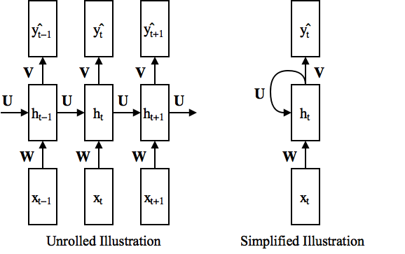
Forward Propagation
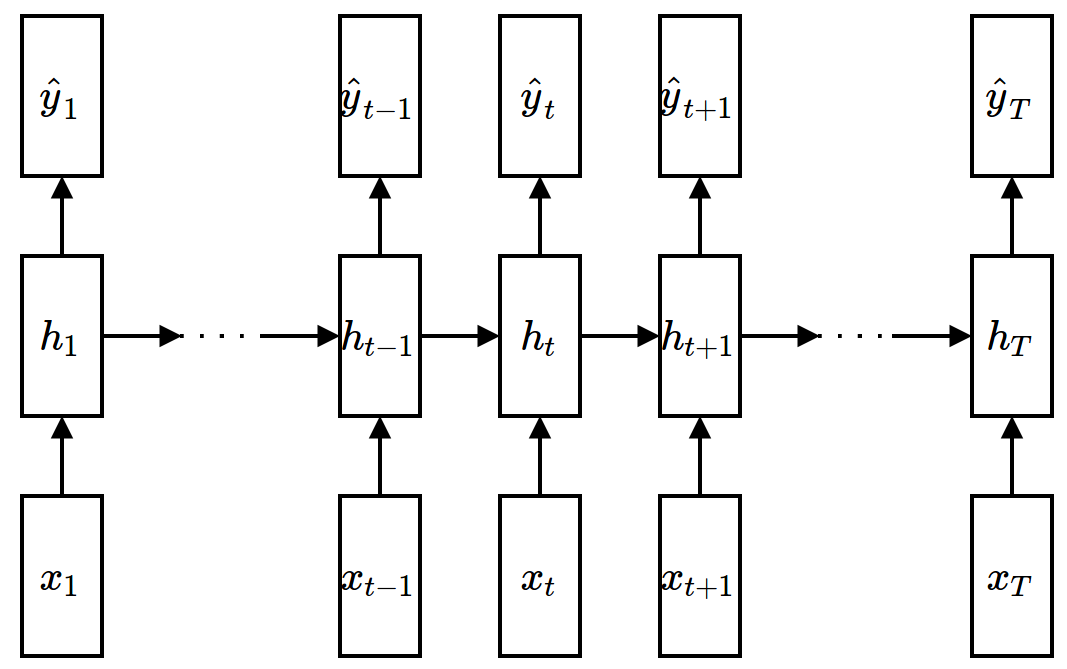
Forward Propagation
$$ \textbf{h}_t = f(\textbf{W}\textbf{x}_t + \textbf{U}\textbf{h}_{t-1}+\textbf{b}) $$$$ \hat{\textbf{y}}_t = \textbf{V}\textbf{h}_t + \textbf{b}' $$$$ \mathcal{L} = \sum_{t=1}^{T} \mathcal{L}_t \left( \textbf{y}_t, \hat{\textbf{y}}_t \right) $$- $\textbf{W}$: input weight, $\textbf{U}$: recurrent weight, $\textbf{V}$: output weight, $\textbf{b},\textbf{b}'$: bias, $f$: non-linear activation (e.g., ReLU)
- Weights are shared across time: the number of parameters does not depend on the length of input/output sequence
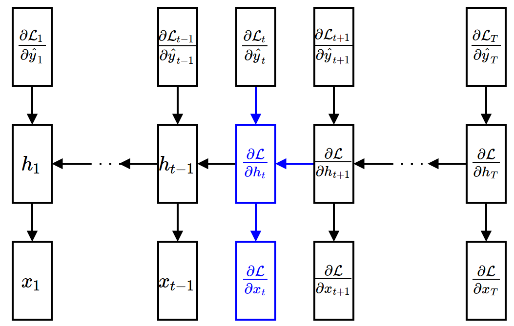
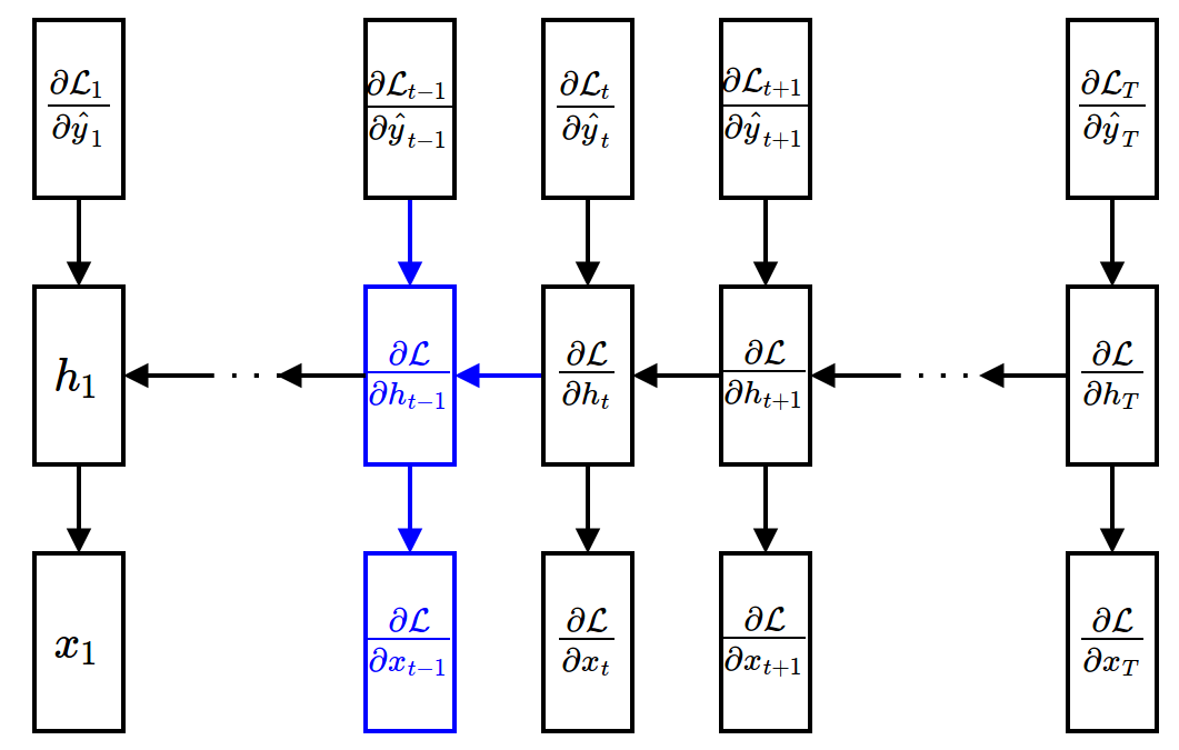
Backpropagation Through Time (BPTT)
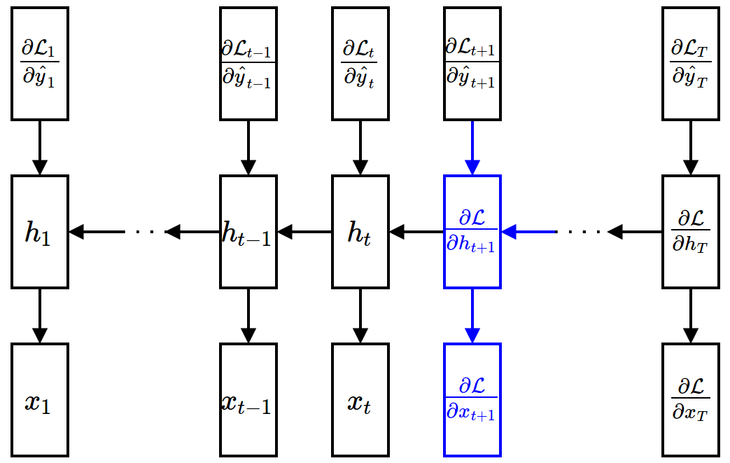
- Gradient w.r.t. hidden units (assuming that $\ppf{\cL}{\vh_{t+1}}$ is given) $$ \begin{align} \frac{\partial\mathcal{L}}{\partial \textbf{h}_t} &= \sum_{\tau=t}^{T}\frac{\partial\mathcal{L}_{\tau}}{\partial \textbf{h}_t} \\ &= \frac{\partial \mathcal{L}_t}{\partial \textbf{h}_t} + \frac{\partial \textbf{h}_{t+1}}{\partial \textbf{h}_{t}} \frac{\partial \sum_{\tau=t+1}^{T}\mathcal{L}_{\tau}}{\partial \textbf{h}_{t+1}} \\ &= \underbrace{\frac{\partial \mathcal{L}_t}{\partial \hat{\textbf{y}}_t}}_{\mbox{easy}}\underbrace{\frac{{\partial \hat{\textbf{y}}_t}}{\partial \textbf{h}_t}}_{\mbox{easy}} + \underbrace{\frac{\partial \textbf{h}_{t+1}}{\partial \textbf{h}_{t}}}_{\mbox{easy}} \underbrace{\frac{\partial \mathcal{L}}{\partial \textbf{h}_{t+1}}}_{\mbox{given}} \end{align} $$
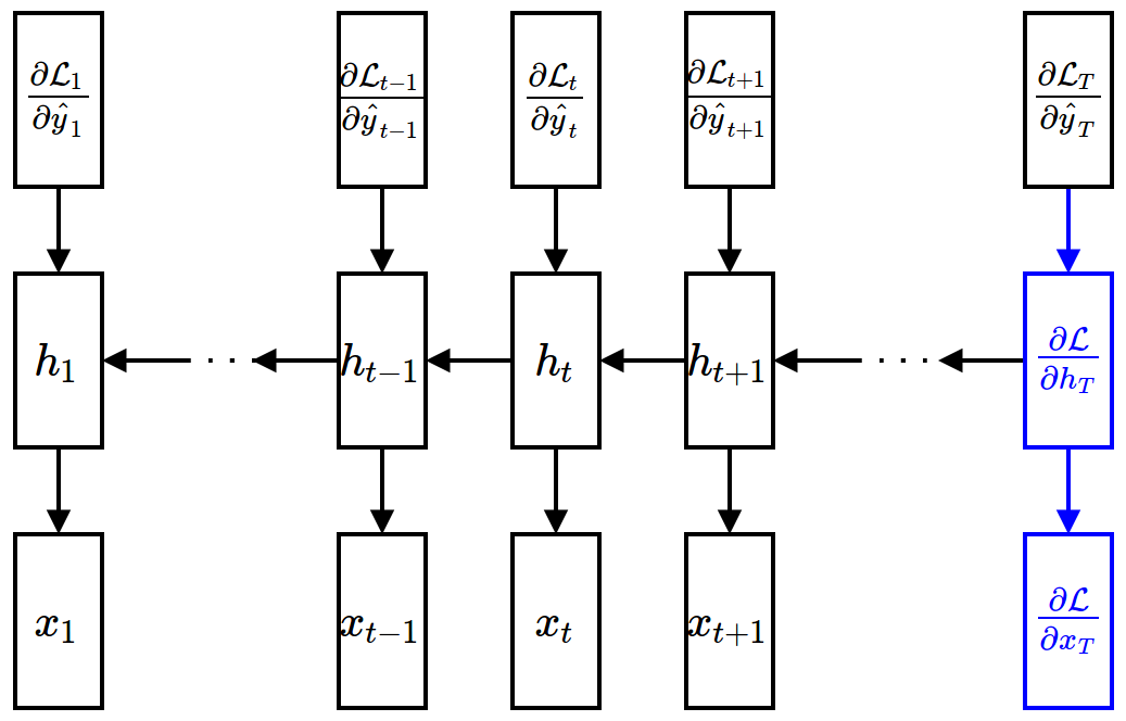
Backpropagation Through Time (BPTT)
- Gradient w.r.t. input units (given $\ppf{\cL}{\vh_t}$)
$$ \frac{\partial\mathcal{L}}{\partial \textbf{x}_t} = \frac{\partial \mathcal{L}}{\partial \textbf{h}_t}\frac{\partial \textbf{h}_t}{\partial \textbf{x}_t} $$
Backward Propagation
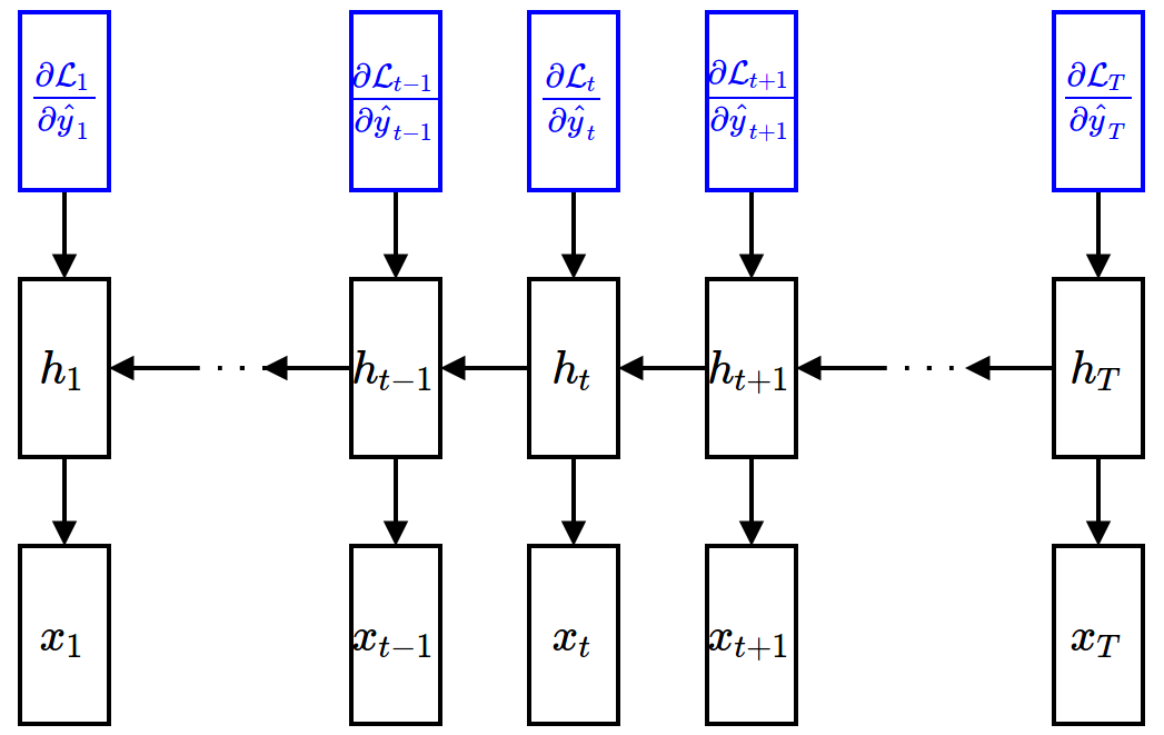
Backward Propagation
Backward Propagation
Backward Propagation
Backward Propagation
Backward Propagation
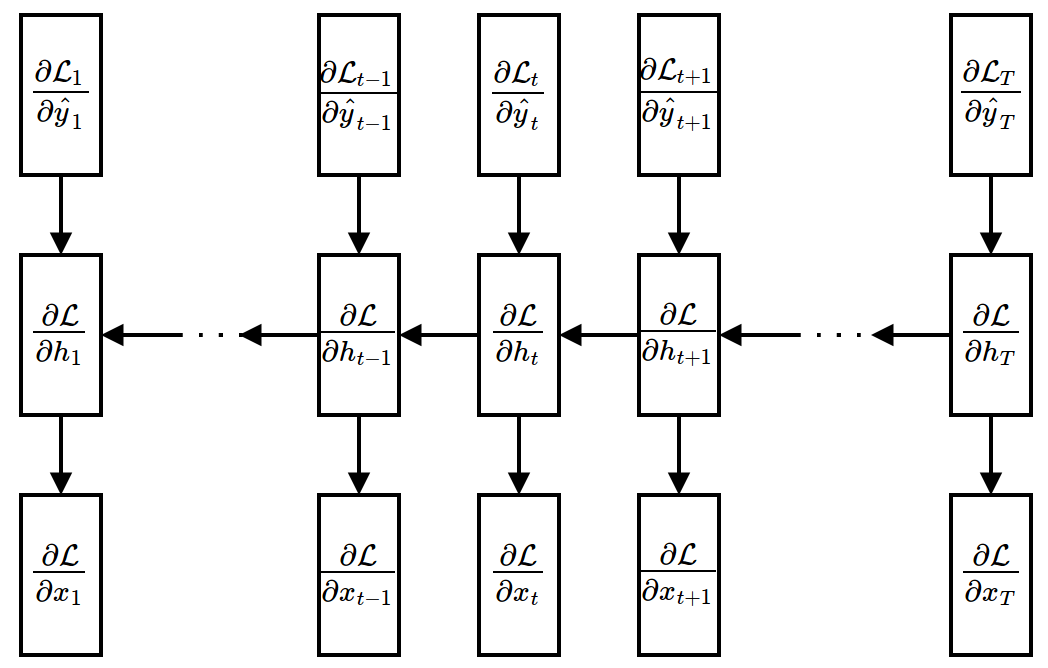
Backpropagation Through Time (BPTT)
- Gradient w.r.t. weights
- Recall: The weights are shared through time. Gradients of shared weights should be accumulated!
Summary of Standard Recurrent Neural Network
- RNN is actually not much different from a standard (feedforward) neural network except that:
- Input/output are given through time.
- Weights are extensively shared.
- RNN can be viewed as a very deep feedforward neural network with shared weights.
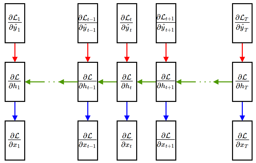
Vanshing Gradient Problem
- RNN can model arbitrary sequences if properly trained.
- In practice, it is difficult to train an RNN to learn long-term dependencies because of vanishing gradient.
- Intuition of vanishing gradient
- A hidden unit activation is not well-preserved to the long-term future (forward propagation view)
- Gradients are diffused through time (backward propagation view)
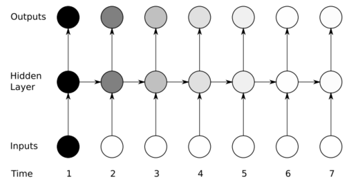 (Figure from Alex Graves)
Mathematical details: Let $\norm{\ppf{\vh_{\tau+1}}{\vh_\tau}}\approx \alpha$
$$ \begin{align} \norm{\ppf{\cL}{\vh_t}} &\propto \norm{\ppf{\vh_{t+1}}{\vh_t}\ppf{\cL}{\vh_{t+1}}} \propto \norm{ \left(\prod_{\tau=t}^{T-1}\ppf{\vh_{\tau+1}}{\vh_\tau}\right) \ppf{\cL}{\vh_T}} \leq \prod_{\tau=t}^{T-1}\norm{\ppf{\vh_{\tau+1}}{\vh_\tau}} \norm{\ppf{\cL}{\vh_T}} \\ \Rightarrow \norm{\ppf{\cL}{\vh_t}} &\approx \alpha^{T-t} \norm{\ppf{\cL}{\vh_T}} \end{align} $$At very old steps, i.e. when $T\gg t$,
- If $\alpha<1$, $\ppf{\cL}{\vh_t} \ll \ppf{\cL}{\vh_T}\quad \Rightarrow$ Gradient vanishing
- If $\alpha>1$, $\ppf{\cL}{\vh_t} \rightarrow \infty\quad \Rightarrow$ Gradient explosion
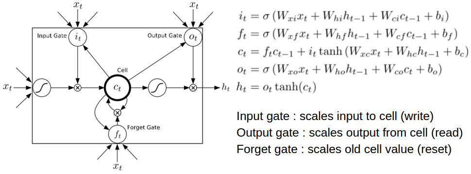
Long Short-Term Memory (LSTM)
- A special type of RNN that can handle vanishing gradient better.
- $i_t,o_t,f_t$: input gate, output gate, and forget gate
- $c_t$: memory cell containing information about history of inputs
- $h_t$: output activation
 (Figure from Alex Graves)
Long Short-Term Memory (LSTM)
- Gating mechanism
- Input gate: whether to ignore a new input or not
- Output gate: whether to produce an output or not (while preserving the memory cell)
- Forget gate: whether to erase the memory cell or not
- Gating is controlled by LSTM's weights that are also learned from data.
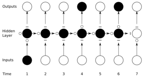 (Figure from Alex Graves)
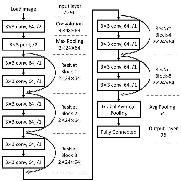
Residual Networks and Infinite-depth Models
The vanishing gradient problem turns out to be universal in deep learning, e.g. in CNN architectures.
This leads to the skip connection technique (which is now standard) and the Residual Network (ResNet).
Ref: Deep Residual Learning for Image Recognition, arXiv 1512.03385 (100k+ citations now...)
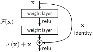
Skip Connection
The ResNet essentially makes the following change: $$ \vx^{(j+1)} = \vF(\vx^{(j)}) \quad\Rightarrow\quad \vx^{(j+1)} = \vx^{(j)} + \vF(\vx^{(j)}) $$ to provide a "bypass" for the back-propagation.
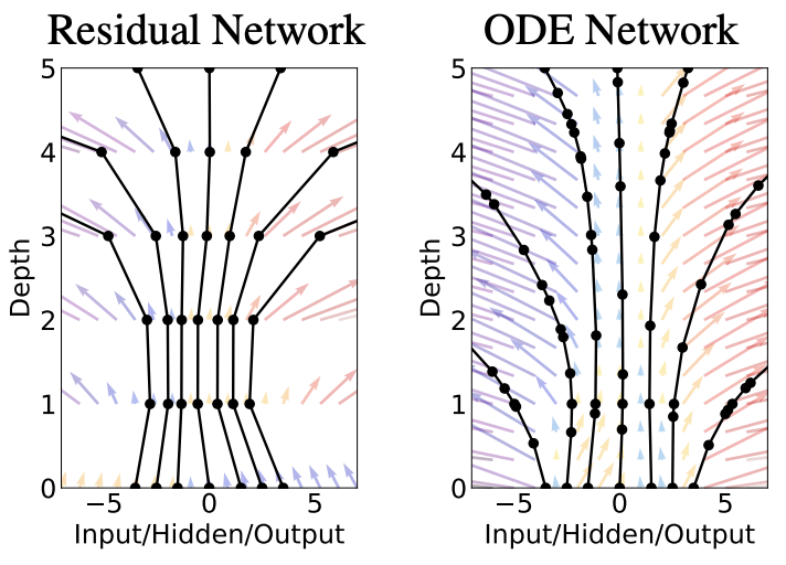
But... Isn't that Euler method?
Recall for a first-order ordinary differential equation (ODE) $$ \dot\vx = \vf(\vx),\quad \vx(0)=\vx_0,\quad t\in[0,T] $$ Forward Euler method with step size $\Delta t$, $\vx_j=\vx(j\Delta t)$ $$ \vx^{j+1} = \vx^{j} + \Delta t\vf(\vx^{j}) $$ Then $\Delta t\vf(\vx^{j})$ is as if the ResNet block $\vF(\vx^{(j)})$ in previous slide!
This leads to Neural ODEs
$$ \dot\vx = \vf(\vx),\quad \vx(0)=\vx_0,\quad t\in[0,T] $$- $\vx_0$ is the input
- $\vf(\vx)$ is a neural network
- $\dot\vx = \vf(\vx)$ governs the forward propagation (think in terms of forward Euler)
- $\vx(T)$ is the output
- $t$ is like the "index" of layers - now infinite!
Ref: Neural Ordinary Differential Equations, arXiv 1806.07366
But ...
- If $\dot\vx = \vf(\vx)$ is the forward propagation
- What is the back-propagation?
- We need the continuous adjoint formulation - to be discussed in the last module.
- There we will generalize NODE to model dynamical systems.
Things not covered
There of course many ... For example
- Time Convolution Network, as an alternative to RNN, for time series modeling
- Autoencoders, for data compression and generation
- We will talk more in the next module
- Generative Adversarial Networks (GAN), e.g., generating "fake" authentic data
- Physics-Informed Neural Network
- Hope to discuss in the last module
And in the bigger picture:
- Network Architecture Search, or more general, Automated Machine Learning (AutoML)
- Automatically determine what network architecture to use
- A simple approach is actually Bayesian optimization from the previous module