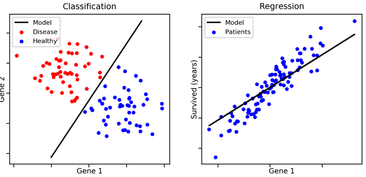
Supervised Learning
- Goal
- Given data $X$ in feature sapce and the labels $Y$
- Learn to predict $Y$ from $X$
- Labels could be discrete or continuous
- Continuous-valued labels: Regression
- Discrete-valued labels: Classification - I don't care
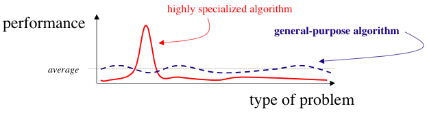
No Free Lunch Theorem
Wolpert and Macready (1997)
We have dubbed the associated results NFL theorems because they demonstrate that if an algorithm performs well on a certain class of problems then it necessarily pays for that with degraded performance on the set of all remaining problems.
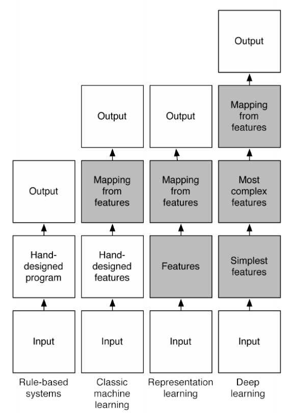
Classical ML v.s. Deep learning
Notation
In this lecture, we will use
- Data $x \in R^D$ (scalar- or vector-valued)
- Features $\phi(x) \in R^M$ for data $x$
- Continuous-valued labels $t \in R$ (target values)
We will interchangeably use
- $x^{(n)}, x_n$ to denote the $n^\text{th}$ training example.
- $t^{(n)}, t_n$ to denote the $n^\text{th}$ target value.
Linear Regression (1d inputs)
- Consider 1d case (e.g. D=1)
- Given a set of observations $x_1, \dots, x_N$
- and corresponding target values $t_1, \dots, t_N$
- We want to learn a function $y(x, \vec{w}) \approx t$ to predict future values.
Regression: Noisy Data
In [3]:
# Truth, without noise
xx, yy = generateData(100, False)

# Noisy observation, training samples
x, y = generateData(13, True)

# plot data
plt.plot(xx, yy, 'g--')
plt.plot(x, y, 'ro')
Out[3]:
[<matplotlib.lines.Line2D at 0x10a41e5e0>]

Regression: 0th Order Polynomial
In [4]:
# Here were are going to take advantage of numpy's 'polyfit' function
# This implements a "polynomial fitting" algorithm
# coeffs are the optimal coefficients of the polynomial
coeffs = np.polyfit(x, y, 0)  # 0 is the degree of the poly

# We construct poly(), the polynomial with "learned" coefficients
poly = np.poly1d(coeffs)

plt.plot(xx, yy, "g--")
plt.plot(x, y, "ro")
plt.plot(xx, poly(xx), "b-")
Out[4]:
[<matplotlib.lines.Line2D at 0x10a502b50>]

Regression: 1st Order Polynomial
In [5]:
coeffs = np.polyfit(x, y, 1) # Now let's try degree = 1
poly = np.poly1d(coeffs)
plt.plot(xx, yy, "g--")
plt.plot(x, y, "ro")
plt.plot(xx, poly(xx), "b-")
Out[5]:
[<matplotlib.lines.Line2D at 0x10a56a370>]

Regression: 3rd Order Polynomial
In [6]:
coeffs = np.polyfit(x, y, 3) # Now degree = 3
poly = np.poly1d(coeffs)

plt.plot(xx, yy, "g--")
plt.plot(x, y, "ro")
plt.plot(xx, poly(xx), "b-")
Out[6]:
[<matplotlib.lines.Line2D at 0x10a5c7730>]

Linear Regression (General Case)
The function $y(\vec{x}, \vec{w})$ is linear in parameters $\vec{w}$.
- Goal: Find the best value for the weights, $\vec{w}$.
- For simplicity, add a bias term $\phi_0(\vec{x}) = 1$.
Basis Functions
The basis functions $\phi_j(\vec{x})$ need not be linear.
In [8]:
r = np.linspace(-1,1,100)
f, axs = plt.subplots(1, 3, figsize=(12,4))
for j in range(8):
    axs[0].plot(r, np.power(r,j))
    axs[1].plot(r, np.exp( - (r - j/7.0 + 0.5)**2 / 2*5**2 ))
    axs[2].plot(r, 1 / (1 + np.exp( - (r - j/5.0 + 0.5) * 5)) )

set_nice_plot_labels(axs) # I'm hiding some helper code that adds labels

Least Squares: Objective Function
Minimize the residual error over the training data.
$$ E(\vec{w}) = \frac12 \sum_{n=1}^N (y(x_n, \vec{w}) - t_n)^2 = \frac12 \sum_{n=1}^N \left( \sum_{j=0}^{M-1} w_j\phi_j(\vec{x}^{(n)}) - t^{(n)} \right)^2 $$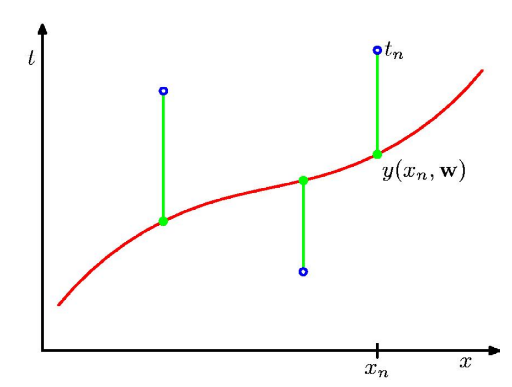
Closed Form Solution: Derivation
$$ \begin{align} \mbox{Scarlar Form: } E(\vec{w}) &= \frac12 \sum_{n=1}^N \left( \sum_{j=0}^{M-1} w_j \phi_j(\vec{x}^{(n)}) - t^{(n)} \right)^2 \\ &= \frac12 \sum_{n=1}^N \left( \vec{w}^T \phi(\vec{x}^n) - t^{(n)} \right)^2 \\ &= \frac12 \sum_{n=1}^N (\vec{w}^T \phi( \vec{x}^{(n)} ) )^2 - \sum_{n=1}^N t^{(n)} \vec{w}^T \phi( \vec{x}^{(n)} ) + \frac12 \sum_{n=1}^N (t^{(n)})^2 \\ \mbox{Vector Form: } E(\vec{w}) &= \frac12 \|\Phi \vec{w} - \vec{t}\|^2 \\ &= \frac12 \vec{w}^T \Phi^T \Phi \vec{w} - \vec{w}^T \Phi^T \vec{t} + \frac12 \vec{t}^T \vec{t} \end{align}$$Closed Form Solution: Data Matrix
The design matrix is a matrix $\Phi \in R^{N \times M}$, applying
- the $M$ basis functions (columns)
- to $N$ data points (rows)
Goal: $\Phi \vec{w} \approx \vec{t}$
Least Squares: Gradient via Matrix Calculus
- Compute the gradient and set to zero
- Solve the resulting normal equation: $$ \Phi^T \Phi w = \Phi^T t \\ w = (\Phi^T \Phi)^{-1} \Phi^T t $$
This is the Moore-Penrose pseudoinverse, $\Phi^\dagger = (\Phi^T \Phi)^{-1} \Phi^T$ applied to solve the linear system $\Phi w \approx t$.
Digression: Moore-Penrose Pseudoinverse
- When we have a matrix $A$ that is non-invertible or not even square, we might want to invert anyway
- For these situations we use $A^\dagger$, the Moore-Penrose Pseudoinverse of $A$
- When $A$ has lin. indep. columns then $A^\dagger = (A^\top A)^{-1} A^\top$
- In general, we can get $A^\dagger$ by SVD: if we write $A = U \Sigma V^\top$ then $A^\dagger = V \Sigma^\dagger U^\top$, where $\Sigma^\dagger$ is obtained by taking reciprocals of non-zero entries of $\Sigma$.
Alternative View: Projection onto subspace
- Columns of $\Phi$ forms a subspace and we are essentially projecting $t$ onto $\Phi$ when doing $\Phi x=t$
- The SVD $\Phi=U\Sigma V^T$ produces the orthonormal basis $U$ and transformation matrix $T=\Sigma V^T$
- Recall from review of linear algebra, let $y=Tx$, then $Uy=t$ and $y\approx U^Tt$
- Then $x=T^{-1}y=V\Sigma^\dagger U^T t=\Phi^\dagger t$
In [10]:
stys = ['k-', 'k-.', 'm-', 'm-.']
plt.plot(xx, yy, "g--")
plt.plot(x, y, "ro", label="Training data")
for _i in range(4):
    plt.plot(xx, tsts[_i], stys[_i], label='Order {0}'.format(_i))
plt.legend()
Out[10]:
<matplotlib.legend.Legend at 0x10a7f8970>

Root of Mean-Squared Error, RMSE
$$ E_{RMS} = \sqrt{2E(w^*) / N} = \sqrt{\frac{1}{N}\sum_{i=1}^N[f(x_i)-t_i]^2} $$- Easy to compute
- Potential issue: Improperly scaled
In [11]:
f, ax = plt.subplots(ncols=4, sharey=True, figsize=(16,4))
for _i in range(4):
    ax[_i].plot(xx, yy, "g--")
    ax[_i].plot(x, y, "ro")
    ax[_i].plot(xx, tsts[_i])
    ax[_i].set_title('Order {0}, RMSE={1:4.3f}'.format(_i, es[_i]))

Coefficient of determination
$$ R^2 = 1 - \frac{SS_{res}}{SS_{tot}} $$- Let $\bar{t}$ be average of $\{t_i\}$
- Residual sum of squares: $$SS_{res}=\sum_i[f(x_i)-t_i]^2$$
- Total sum of squares: $$SS_{tot}=\sum_i[t_i-\bar{t}]^2$$
- Explained sum of squares: $$SS_{reg}=\sum_i[f(x_i)-\bar{t}]^2$$
In [12]:
f, ax = plt.subplots(ncols=4, sharey=True, figsize=(16,4))
for _i in range(4):
    ax[_i].plot(y, y, "r-")
    ax[_i].plot(y, trns[_i], "bo")
    ax[_i].set_title('Order {0}, R2={1:4.3f}'.format(_i, rs[_i]))

Geometrical interpretation of R2
- Blue: Squared residuals w.r.t. the linear regression.
- Red: Squared residuals w.r.t. the average value.

In [ ]: