Previously: Curve-fitting examples...
- Consider 1d case (e.g. D=1)
- Given a set of observations $x_1, \dots, x_N$
- and corresponding target values $t_1, \dots, t_N$
- We want to learn a function $y(x, \vec{w}) \approx t$ to predict future values.
0th Order Polynomial
coeffs = np.polyfit(x, y, 0)
poly = np.poly1d(coeffs)
plt.plot(xx, yy, "g--")
plt.plot(x, y, "ro")
_=plt.plot(xx, poly(xx), "b-")

3rd Order Polynomial
coeffs = np.polyfit(x, y, 3)
poly = np.poly1d(coeffs)
plt.plot(xx, yy, "g--")
plt.plot(x, y, "ro")
_=plt.plot(xx, poly(xx), "b-")

12th Order Polynomial
coeffs = np.polyfit(x, y, 12)
poly = np.poly1d(coeffs)
plt.plot(xx, yy, "g--")
plt.plot(x, y, "ro")
_=plt.plot(xx, poly(xx), "b-")

Overfitting
Root-Mean-Square (RMS) Error: $E_{RMS} = \sqrt{2E(w^*) / N} = \sqrt{\frac{1}{N}\sum_{i=1}^N[f(x_i)-t_i]^2}$
f = plt.figure()
plt.plot(_ps, _trns, 'bo-', label='Training error')
plt.plot(_ps, _tsts, 'rs-', label='Test error')
plt.legend()
plt.xlabel("Order of polynomial")
_=plt.ylabel("RMSE")

Polynomial Coefficients
for _s in _d:
    print(_s)
w0      0.66712    -0.06918     0.10366     0.12353
w1     -0.22739     1.66469     0.04525   156.79232
w2                 -0.80783     1.39030  -874.67537
w3                  0.08731    -1.05527  2007.14361
w4                              0.27977 -2543.62965
w5                             -0.03264  2006.68009
w6                              0.00147 -1045.52459
w7                                        369.91998
w8                                        -89.40320
w9                                         14.53250
w10                                         -1.51902
w11                                          0.09219
w12                                         -0.00247
Data Set Size: $N = 15$
(12th order polynomial)
# New trainging set
x1, y1 = generateData(15, True)
# fit
coeffs = np.polyfit(x1, y1, 12)
poly = np.poly1d(coeffs)
_=plt.plot(xx, yy, "g--", x1, y1, "ro", xx, poly(xx), "b-")

Data Set Size: $N = 100$
(12th order polynomial)
# New trainging set
x2, y2 = generateData(100, True)
# fit
coeffs = np.polyfit(x2, y2, 12)
poly = np.poly1d(coeffs)
_=plt.plot(xx, yy, "g--", x2, y2, "ro", xx, poly(xx), "b-")

How do we choose the degree of our polynomial?
AKA number of features
Numerically, the issue traces back to the "conditioning" of the $\Phi^T\Phi$ matrix.
- Recall $\kappa(A)=|A^{-1}||A|$ as the condition number of $A$, $\kappa(A)$.
- One wants $\kappa(A)$ close to 1 for "numerically stable" solutions for $Ax=b$.
Example: Solve for $x=A^{-1}b$ $$ A=\begin{bmatrix}2\alpha & 1 \\ 1 & \frac{2}{\alpha}\end{bmatrix},\quad b=[1,10^{10}] $$ and we verify if we recover $b$ by doing $b=Ax=AA^{-1}b$.
kA = lambda a: np.linalg.cond([[2*a,1.],[1.,2/a]])
a = 10**np.linspace(1,11,21)
k = [kA(_) for _ in a]
plt.loglog(a, k)
plt.xlabel(r'$\alpha$')
_=plt.ylabel(r'$\kappa(A)$')

fA = lambda a: np.array([[2*a,1.],[1.,2./a]])
sA = lambda a: fA(a).dot(np.linalg.solve(fA(a), [1,1e10]))[0]
a = 10**np.linspace(1,11,21)
s = [sA(_) for _ in a]
plt.semilogx(a, np.ones_like(a), 'r--', label='Expected')
plt.semilogx(a, s, 'b-', label='Numerical')
plt.xlabel(r'$\alpha$')
plt.ylabel(r'First element of $AA^{-1}b$')
_=plt.legend()

Rule of Thumb - I
- First of all, normalize your data
- For example, Scale to [0,1] using max and min, or Scale using mean and std $$\hat{x}=\frac{x-x_{\min}}{x_{\max}-x_{\min}},\quad\mbox{or}\quad \hat{x}=\frac{x-\mu}{\sigma}$$
- Scale input only, or both input and output, depending on the bias
- If you scaled the output, remember to scale the predicted output back when using your trained model.
- The min/max or mean/std should be computed from the training dataset only
Rule of Thumb - II
- Keep a tall-and-thin shape of the design matrix $\Phi$ for better conditioning - which means,
- For a small number of datapoints, use a low degree
- Otherwise, the model will overfit!
- As you obtain more data, you can gradually increase the degree
- Add more features to represent more data
- Warning: Your model is still limited by the finite amount of data available.
Or -
- Use regularization to control model complexity.
Regularized Linear Regression
Regularized Least Squares
- Consider the error function $E_D(w) + \lambda E_W(w)$
- Data term $E_D(w)$
- Regularization term $E_W(w)$
- With the sum-of-squares error function and quadratic regularizer, $$ \widetilde{E}(w) = \frac12 \sum_{n=1}^N (y(x_n, w) - t_n)^2 + \boxed{\frac{\lambda}{2} || w ||^2} $$
- This is minimized by $$ w = (\lambda I + \Phi^T \Phi)^{-1} \Phi^T t $$
Regularized Least Squares: Derivation
Recall that our objective function is
\begin{align} E(w) &= \frac12 \sum_{n=1}^N (w^T \phi(x^{(n)}) - t^{(n)})^2 + \frac{\lambda}{2} w^T w \\ &= \frac12 w^T \Phi^T \Phi w - w^T \Phi^T t + \frac12 t^T t + \frac{\lambda}{2} w^T w \end{align}Regularized Least Squares: Derivation
Compute gradient and set to zero:
$$ \begin{align} \nabla_w E(w) &= \nabla_w \left[ \frac12 w^T \Phi^T \Phi w - w^T \Phi^T t + \frac12 t^T t + \frac{\lambda}{2} w^T w \right] \\ &= \Phi^T \Phi w - \Phi^T t + \lambda w \\ &= (\Phi^T \Phi + \lambda I) w - \Phi^T t = 0 \end{align} $$Therefore, we get $\boxed{w_{ML} = (\Phi^T \Phi + \lambda I)^{-1} \Phi^T t}$
Regularized Least Squares: Norms
We can make use of the various $L_p$ norms for different regularizers:
$$ \widetilde{E}(w) = \frac12 \sum_{n=1}^N (t_n - w^T \phi(x_n))^2 + \frac{\lambda}{2} \sum_{j=1}^M |w_j|^q $$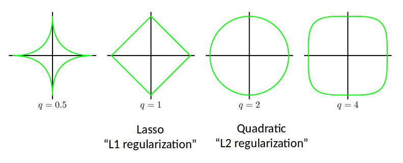
L2 regularization is also called Ridge Regression.
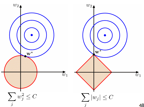
Regularized Least Squares: Comparison
- At the solution the contours are always tangent to each other.
- Lasso tends to generate sparser solutions than a quadratic regularizer.
Another explanation for L2 regularization, using Fourier analysis: https://arxiv.org/abs/1806.08734v1
Examples: Regularized regression
Ridge Regression
rdg_sc, rdg_coef = fitModel(1.0, lm.Ridge)

Lasso
las_sc, las_coef = fitModel(0.01, lm.Lasso)

LR vs Ridge vs Lasso
ii = np.arange(13)
f = plt.figure(figsize=(8,6))
plt.semilogy(ii, np.abs(_cs[11]), 'r--', label='LR')
plt.semilogy(ii, np.abs(rdg_coef), 'b-', label='Ridge')
plt.semilogy(ii, np.abs(las_coef), 'g-', label='Lasso')
plt.legend()
_=plt.xlabel(r'$w_i$')

Bad choice of hyperparameter
_, _ = fitModel(1e-8, lm.Ridge)

_, _ = fitModel(1e8, lm.Ridge)

Choosing the best hyperparameter
f = plt.figure()
plt.plot(np.log(lams), errs[0], 'b-', label='Training error')
plt.plot(np.log(lams), errs[1], 'r-', label='Test error')
plt.xlabel(r'$\log(\lambda)$')
_=plt.ylabel('1-R2')

Regularized Least Squares: Summary
- Simple modification of linear regression
- L2 Regularization controls the tradeoff between fitting error and complexity.
- Small L2 regularization results in complex models, but with risk of overfitting
- Large L2 regularization results in simple models, but with risk of underfitting
- It is important to find an optimal regularization that balances between the two
- More on model selection in future lectures
One more model... Elastic net
- Combination of Ridge and Lasso $$ \widetilde{E}(w) = \frac12 \sum_{n=1}^N (t_n - w^T \phi(x_n))^2 + \lambda\left( \frac{1-\alpha}{2} \sum_{j=1}^M |w_j|^2 + \alpha\sum_{j=1}^M |w_j| \right) $$
- Works better when the features are correlated.
- More details:
- [MLaPP] Chp. 13.5.3
- H. Zou and T. Hastie, Regularization and variable selection via the elastic net, 2005
Yet more models...
The bias of the Lasso estimate for a truly nonzero variable is about $\lambda$ for large regression coefficients coefficients.
To fix the issue: Adaptive Lasso, MCP, SCAD
- for those who are interested: https://myweb.uiowa.edu/pbreheny/7600/s16/notes/2-29.pdf
When it comes to deep learning
We will see Double-Descent phenomenon - Errors in training and test both decrease as number of features increase.
To be discussed more in L7.