Locally-Weighted Linear Regression
Locally-Weighted Linear Regression
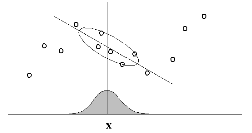
Main Idea: When predicting $f(x)$, give high weights for neighbors of $x$.
Regular vs. Locally-Weighted Linear Regression
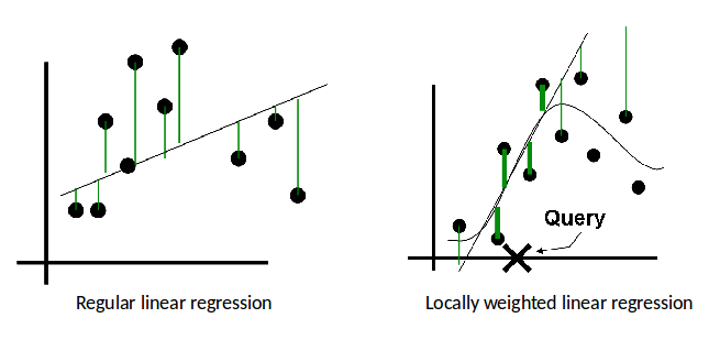
Regular vs. Locally-Weighted Linear Regression
Linear Regression
2. Output $w^T \phi(x_k)$
Locally-weighted Linear Regression
2. Output $w^T \phi(x_k)$
Locally-Weighted Linear Regression
- The standard choice for weights $r$ uses the Gaussian Kernel, with kernel width $\tau$ $$ r_k = \exp\left( -\frac{|| x_k - x ||^2}{2\tau^2} \right) $$
- Note $r_k$ depends on both $x$ (query point); must solve linear regression for each query point $x$.
- Can be reformulated as a modified version of least squares problem.
The formulation and implementation are left for HW1.
Locally-Weighted Linear Regression
- Choice of kernel width matters.
- (requires hyperparameter tuning!)
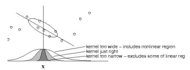
The estimator is minimized when kernel includes as many training points as can be accomodated by the model. Too large a kernel includes points that degrade the fit; too small a kernel neglects points that increase confidence in the fit.
Kernel Method
Review: Feature Mapping
Our models so far employ a nonlinear feature mapping $\phi : \mathcal{X} \mapsto \R^M$
- in general, features are nonlinear functions of the data
- each feature $\phi_j(x)$ extracts important properties from $x$
Allows us to use linear methods for nonlinear tasks.
- For example, polynomial features for linear regression...
Linear Regression: Polynomial Features
Problem: Linear model $y(x) = w^T x$ can only produce straight lines through the origin.
- Not very flexible / powerful
- Can't handle nonlinearities
Solution: Polynomial Regression
- Replace $x$ by $\phi(x) = [1, x, x^2, \cdots, x^p]^T$
- The feature mapping $\phi$ is nonlinear
Linear Regression: Polynomial Features
# ground truth:  function to be approximated
def fn(x): return np.sin(x)

# plot
poly_reg_example(fn)

Linear Regression: Nonlinear Features
Linear Regression Model $$ y(x,w) = w^T \phi (x) = \sum_{j=0}^{M} w_j \phi_j(x) $$
Ridge Regression $$ J(w) = \frac{1}{2} \sum_{n=1}^{N}(w^T \phi (x_n) - t_n)^2 + \frac{\lambda}{2}w^Tw $$
Closed-form Solution $$ w = (\phi^T \phi + \lambda I)^{-1}\phi^T t $$
This is neat, but...
How do I choose a feature mapping $\phi(x)$?
- Manually? Learn features?
With $N$ examples and $M$ features,
- design matrix is $\Phi \in \R^{N \times M}$
- linear regression requires inverting $\Phi^T \Phi \in \R^{M \times M}$
- computational complexity of $O(M^3)$
Feature Mapping: Example
Problem: Find proper features for the following scattered data
plot_circular_data(100)

Feature Mapping: Example
Solution 1: Add squared-distance-to-origin $(x_1^2 + x_2^2)$ as third feature.
plot_circular_3d(100)

Feature Mapping: Example
Solution 2: Replace $(x_1, x_2)$ with $(x_1^2, x_2^2)$
plot_circular_squared(100)

Feature Mapping: Discussion
Data has been mapped via $\phi$ to a new, higher-dimensional (possibly infinite!) space
- Certain representations are better for certain problems
Alternatively, the data still lives in original space, but the definition of distance or inner product has changed.
- Certain inner products are better for certain problems
Feature Mapping: Discussion
Unfortunately, higher-dimensional features come at a price!
- We can't possibly manage infinite-dimensional $\phi(x)$!
- Computational complexity blows up.
Kernel methods to the rescue!
Kernel Methods: Intro
Many algorithms depend on the data only through pairwise inner products between data points, $$ \langle x_1, x_2 \rangle = x_2^T x_1 $$
Inner products can be replaced by Kernel Functions, capturing more general notions of similarity.
- No longer need coordinates!
Kernel Functions: Definition
A kernel function $\kappa(x,x’)$ is intended to measure the similarity between $x$ and $x’$.
So far, we have used the standard inner product in the transformed space, $$ \kappa(x, x') = \phi(x)^T \phi(x') $$
In general, $\kappa(x, x')$ is any symmetric positive-semidefinite function. This means that for every set $x_1, ..., x_n$, the matrix $[\kappa(x_i,x_j)]_{i,j\in[n]}$ is a PSD matrix.
Kernel Functions: Implicit Feature Map
For every valid kernel function $\kappa(x, x')$,
- there is an implicit feature mapping $\phi(x)$
- corresponding to an inner product $\phi(x)^T \phi(x')$ in some high-dimensional feature space
This incredible result follows from Mercer's Theorem,
- Generalizes the fact that every positive-definite matrix corresponds to an inner product
- For more info, see Reproducing Kernel Hilbert Space
Kernel Functions: Simple Example
Kernel: For $x = (x_1, x_2)$ and $z=(z_1, z_2)$, define $$ \begin{align} \kappa(x, z) &= (x^Tz)^2 \\ &= (x_1z_1 + x_2z_2)^2 \\ &= x_1^2z_1^2 + 2x_1z_1x_2z_2 + x_2^2z_2^2 \end{align} $$
Mapping: Equivalent to the standard inner product when either $$ \begin{gather} \phi(x) = (x_1^2, \sqrt{2} x_1 x_2, x_2^2) \\ \phi(x) = (x_1^2, x_1 x_2, x_1 x_2, x_2^2) \end{gather} $$
Implicit mapping is not unique!
Kernel Functions: Polynomial Example
Kernel: Higher-order polynomial of degree $p$, $$ \kappa(x,z) = (x^T z)^p = \left( \sum_{k=1}^M x_k z_k \right)^p $$
Mapping: Implicit feature vector $\phi(x)$ contains all monomials of degree $p$
Kernel Functions: Polynomial Example
Kernel: Inhomogeneous polynomial up to degree $p$, for $c > 0$, $$ \kappa(x,z) = (x^T z + c)^p = \left(c + \sum_{k=1}^M x_k z_k \right)^p $$
Mapping: Implicit feature vector $\phi(x)$ contains all monomials of degree $\leq p$
Example: CFD solution
Take the pixel values and compute $\kappa(x,z) = (x^Tz + 1)^p $
- here, $x$ = $449 \times 129 \approx 60k$ nodes, (From NASA Langley)
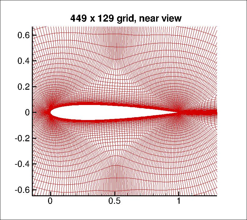
You can compute the inner product in the space of all monomials up to degree $p$
- For $dim(x)\approx 60k$ and $p=3$ a $32T$ dimensional space!
The Kernel Trick
- By using different definitions for inner product, we can compute inner products in a high dimensional space, with only the computational complexity of a low dimensional space.
- Many algorithms can be expressed completely in terms of kernels $\kappa(x,x’)$, rather than other operations on $x$.
- In this case, you can replace one kernel with another, and get a new algorithm that works over a different domain.
Dual Representation and Kernel Trick
The dual representation, and its solutions, are entirely written in terms of kernels.
The elements of the Gram matrix $ K =\Phi \Phi^T $ $$ K_{ij} = \kappa(x_i, x_j) = \phi(x_i)^T \phi(x_j) $$
These represent the pairwise similarities among all the observed feature vectors.
- We may be able to compute the kernels more efficiently than the feature vectors.
Kernel Substitution
To use the kernel trick, we must formulate (training and test) algorithms purely in terms of inner products between data points
We cannot access the coordinates of points in the high-dimensional feature space
This seems a huge limitation, but it turns out that quite a lot can be done
Example: Distance
Distance between samples can be expressed in inner products: $$ \begin{align} ||\phi(x) - \phi(z) ||^2 &= \langle\phi(x)- \phi(z), \phi(x)- \phi(z) \rangle\\ &= \langle \phi(x), \phi(x)\rangle - 2\langle\phi(x), \phi(z)\rangle + \langle\phi(z), \phi(z) \rangle \\ &= \kappa(x,x) - 2\kappa(x,z) + \kappa(z,z) \end{align} $$
Example: Mean
Question: Can you determine the mean of data in the mapped feature space through kernel operations only?
Answer: No, you cannot compute any point explicitly.
Example: Distance to the Mean
Mean of data points given by: $\phi(s) = \frac{1}{N}\sum_{i=1}^{N}\phi(x_i)$
Distance to the mean: $$ \begin{align} ||\phi(x) - \phi_s ||^2 &= \langle\phi(x)- \phi_s, \phi(x)- \phi_s \rangle\\ &= \langle \phi(x), \phi(x)\rangle - 2\langle\phi(x), \phi_s\rangle + \langle\phi_s, \phi_s \rangle \\ &= \kappa(x,x) - \frac{2}{N}\sum_{i=1}^{N}\kappa(x,x_i) + \frac{1}{N^2}\sum_{j=1}^{N}\sum_{i=1}^{N}\kappa(x_i,x_j) \end{align} $$
Constructing Kernels
Method 1: Explicitly define a feature space mapping $\phi(x)$ and use inner product kernel $$ \kappa(x,x') = \phi(x)^T \phi(x') = \sum_{i=1}^{M}\phi_i(x) \phi_i(x') $$
Constructing Kernels
Method 2: Explicitly define a kernel $\kappa(x,x')$ and identify the implicit feature map, e.g. $$ \kappa(x,z) = (x^Tz)^2 \quad \implies \quad \phi(x) = (x_1^2, \sqrt{2} x_1 x_2, x_2^2) $$
Kernels help us avoid the complexity of explicit feature mappings.
Constructing Kernels
Method 3: Define a similarity function $\kappa(x, x')$ and use Mercer's Condition to verify that an implicit feature map exists without finding it.
- Define the Gram matrix $K$ to have elements $K_{nm} = \kappa(x_n,x_m)$
- $K$ must positive semidefinite for all possible choices of the data set {$x_n$} $$ a^TKa \equiv \sum_{i}\sum_{j} a_i K_{ij} a_j \geq 0 \quad \forall\, a \in \R^n $$
Constructing Kernels: Building Blocks
There are a number of axioms that help us construct new, more complex kernels, from simpler known kernels.
- For example, the following are kernels: $$ \begin{align} \kappa(x, x') &= f(x) \kappa_1(x,x') f(x') \\ \kappa(x, x') &= \exp( \kappa_1(x, x') ) \\ \kappa(x, x') &= \exp\left( - \frac{|| x - x' ||^2 }{2\sigma^2} \right) \end{align} $$
Popular Kernel Functions
Simple Polynomial Kernel (terms of degree $2$) $$\kappa(x,z) = (x^Tz)^2 $$
Generalized Polynomial Kernel (degree $M$) $$\kappa(x,z) = (x^Tz + c)^M, c > 0 $$
Gaussian Kernels $$ \kappa(x,z) = \exp \left\{-\frac{||x-z||^2}{2\sigma^2} \right\} $$
Gaussian Kernel
Not related to Gaussian PDF!
Translation invariant (depends only on distance between points)
Corresponds to an infinitely dimensional space!
Dual Representations: Ridge Regression
We want to min: $J(w) = \frac{1}{2} \sum_{n=1}^{N}(w^T \phi (x_n) - t_n)^2 + \frac{\lambda}{2}w^Tw$
Taking $\nabla J(w) = 0$, we obtain: $$ \begin{align} w &= -\frac{1}{\lambda}\sum_{n=1}^{N}(w^T\phi(x_n) - t_n) \phi(x_n) \\ &= \sum_{n=1}^{N}a_n\phi(x_n) = \Phi^Ta \end{align} $$ Notice: $w$ can be written as a linear combination of the $\phi(x_n)$!
Transform $J(w)$ to $J(a)$ by substituting $ w = \Phi^T a$
- Where $a_n = -\frac{1}{\lambda}\left\{w^T\phi(x_n) - t_n)\right\}$
- Let $a = (a_1, \dots, a_N)^T$ be the parameter, instead of $w$.
Dual Representations: Ridge Regression
Dual: Substituting $w = \Phi^Ta$, $$ \begin{align} J(a) &= \frac12 w^T \Phi^T \Phi w - w^T \Phi^T t + \frac12 t^T t + \frac{\lambda}{2} w^T w \\ &= \frac{1}{2} (a^T\Phi) \Phi^T \Phi (\Phi^Ta) - (a^T\Phi) \Phi^Tt + \frac{1}{2}t^Tt + \frac{\lambda}{2}(a^T\Phi)(\Phi^Ta) \\ &= \frac{1}{2} a^T \color{red}{(\Phi \Phi^T) (\Phi \Phi^T)} a - a^T \color{red}{(\Phi\Phi^T)} t + \frac{1}{2}t^Tt + \frac{\lambda}{2}a^T \color{red}{(\Phi\Phi^T)} a \\ &= \frac{1}{2}a^TKKa - a^T Kt + \frac{1}{2}t^Tt + \frac{\lambda}{2}a^TKa \end{align} $$
Dual Representations: Ridge Regression
Dual: Substituting $w = \Phi^Ta$, $$ J(a) = \frac{1}{2}a^TKKa - a^T Kt + \frac{1}{2}t^Tt + \frac{\lambda}{2}a^TKa $$ Prediction: Hypothesis becomes $$ y(x) = w^T\phi(x) = a^T \Phi\phi(x) = a^T \mathbf{k}(x) $$ where $$ \mathbf{k}(x) = \Phi \phi(x) = [k(x_1,x), \ldots, k(x_n,x)]^T $$ We still need to solve for $a$!
Dual Representations: Summary
- Transform $J(w)$ to $J(a)$ by using $w = \Phi^Ta$ and the Gram matrix $K = \Phi\Phi^T$
- Find $a$ to minimize $J(a)$ $$ \boxed{a = (K+\lambda I_N)^{-1}t} $$
- For predictions (for query point/test example x)
$$
y(x)
= w^T\phi(x)
= a^T \Phi\phi(x)
= \mathbf{k}(x)^T (K+\lambda I_N)^{-1}t
$$
- where $\mathbf{k}(x)$ has elements $\kappa(x_1, x), \ldots, \kappa(x_n,x)$
- This leads to Kernel Regression
Dual Representations: Primal vs. Dual
Primal: $w = (\Phi^T\Phi + \lambda I_M)^{-1} \Phi^Tt $
- invert $\Phi^T \Phi \in \R^{M \times M}$
- cheaper since usually $N >> M$
- must explicitly construct features
Dual: $ a = (K + \lambda I_N)^{-1}t $
- invert Gram matrix $K \in \R^{N \times N}$
- use kernel trick to avoid feature construction
- use kernels $\kappa(x, x')$ to represent similarity over vectors, images, sequences, graphs, text, etc..
Kernel Regression: Example
$\kappa(x,y)=\exp(-\gamma||x-y||^2)$
Kernel Regression: Linear + Noise
n = 20
# linear + noise
X = np.linspace(0,10,n).reshape(-1,1)
y = (X + np.random.randn(n,1)).reshape(-1)
# plot
plot_kernel_ridge(X, y, gamma=4, alpha=0.01)

Kernel Regression: Sine + Linear + Noise
n = 30
# Sine + linear + noise
X = np.linspace(0,10,n).reshape(-1,1)
y = (2*np.sin(2*X) + X + np.random.randn(n,1)).reshape(-1)
# plot
plot_kernel_ridge(X, y, gamma=0.5, alpha=0.01)

Kernel Regression: Completely Random
n = 30
# completely random
X = np.linspace(0,10,n).reshape(-1,1)
y = np.random.randn(n,)
# plot
plot_kernel_ridge(X, y, gamma=0.5, alpha=0.01)

Comparison to Locally-Weighted Linear Regression
Locally-weighted Linear Regression
2. Output $w(x)^T \phi(x)$
Use Gaussian Kernel, $r_n(x) = \exp \left\{-\frac{||x- x_n||^2}{2\sigma^2} \right\}$
Comparison to Locally-Weighted Linear Regression
Similarities: Both methods are “instance-based learning”, i.e. non-parametric method
- Only observations (training set) close to the query point are considered (highly weighted) for regression computation.
- Kernel determines how to assign weights to training examples (similarity to the query point x)
- Free to choose types of kernels
- Both can suffer when the input dimension is high.
Comparison to Locally-Weighted Linear Regression
Differences:
- LWLR: Weighted regression; slow, but more accurate
- KR: Weighted mean; faster, but less accurate