An incomplete review.

Introduction

In a previous article, we discussed Bayesian optimization for single objective problems. This article will discuss the multi-objective optimization (MO) and provide a partial review of the classical and the Bayesian MO algorithms.

Defining a multi-objective optimization

Some of the mathematical contents follow this lecture note.

Formally, an MO is written as, $\displaystyle \begin{aligned} {\mathop{\mathrm{arg\,min}}\limits_{\mathbf{x}}} &\quad {\mathbf{f}}({\mathbf{x}})=[f_1({\mathbf{x}}),\cdots,f_n({\mathbf{x}})] \\ {\mathrm{s.t.}}&\quad {\mathbf{c}}_E({\mathbf{x}}) = 0 \\ &\quad {\mathbf{c}}_I({\mathbf{x}}) \ge 0 \\ &\quad {\mathbf{x}}_{lb} \le {\mathbf{x}}\le {\mathbf{x}}_{ub} \end{aligned}$ or simply writing the constraints as ${\mathbf{x}}\in{\mathcal{X}}$, where ${\mathcal{X}}$ is the feasible design space.

Assume that $f_i^*$ is the minimum attainable value of the $i$th objective in the feasible design space, i.e. $f_i^*$ is the solution to the single-objective optimization (SO) consisting of the $i$th objective and all the constraints of the MO. The collection of all these solutions ${\mathbf{f}}^*=[f_1^*,\cdots,f_n^*]$ is defined as the ideal objective vector. In a typical MO problem, such a point is not attainable. That means no single solution exists that simultaneously optimizes each objective – this is the fundamental problem in MO.

When ${\mathbf{f}}^*$ is unattainable, the objective functions are said to be conflicting and there exists a (possibly infinite) number of Pareto optimal solutions. A solution is called Pareto optimal if none of the objectives can be decreased without increasing some of the other objectives. Two Pareto optimal solutions are mutually nondominated. That means there exists some objectives in one solution that are smaller than those in the other solution.

The dominance is more precisely defined via the partial ordering, or the dominance relation between the design vectors ${\mathbf{x}}$. ${\mathbf{x}}_1$ dominates ${\mathbf{x}}_2$, denoted ${\mathbf{x}}_1\preceq{\mathbf{x}}_2$, if (1) $f_i({\mathbf{x}}_1)\leq f_i({\mathbf{x}}_2)$ for $i=1,\cdots,n$ and (2) $\exists j\in \{ 1,\cdots,n\}$, $f_j({\mathbf{x}}_1)< f_j({\mathbf{x}}_2)$. The corresponding objective vectors are denoted ${\mathbf{f}}_1\preceq{\mathbf{f}}_2$. The dominance is strict, denoted ${\mathbf{x}}_1\prec{\mathbf{x}}_2$ and ${\mathbf{f}}_1\prec{\mathbf{f}}_2$, if (2) is true for all $j$’s.

Using the dominance relation, a solution ${\mathbf{x}}$ is (1) globally Pareto optimal if ${\mathbf{x}}\preceq{\mathbf{x}}'$, $\forall{\mathbf{x}}'\in{\mathcal{X}}$, (2) locally Pareto optimal if $\exists\epsilon$, ${\mathbf{x}}\preceq{\mathbf{x}}'$, $\forall{\mathbf{x}}',\lVert{\mathbf{x}}-{\mathbf{x}}'\rVert<\epsilon$. All globally (locally) Pareto optimal solutions form the global (local) Pareto set ${\mathcal{X}}^p$ and its image in the objective space is the global (local) Pareto front ${\mathcal{F}}$.

The ideal objective vector ${\mathbf{f}}^*$ is more formally defined by setting its $i$th entry to be $\displaystyle [{\mathbf{f}}^*]_i = \inf_{ {\mathbf{x}}\in{\mathcal{X}}^p } f_i({\mathbf{x}}),\quad i=1,\cdots,n$ Similarly, the nadir objective vector ${\mathbf{f}}^n$ is defined by setting its $i$th entry to be $\displaystyle [{\mathbf{f}}^n]_i = \sup_{ {\mathbf{x}}\in{\mathcal{X}}^p } f_i({\mathbf{x}}),\quad i=1,\cdots,n$ The ideal and nadir objective vectors define the lower and upper bounds of the Pareto front and thus can be used for normalization. The $i$th entry of the normalized objective vector is $\displaystyle [\bar{ {\mathbf{f}}}^p]_i = \frac{ [{\mathbf{f}}^p]_i-[{\mathbf{f}}^*]_i }{ [{\mathbf{f}}^n]_i-[{\mathbf{f}}^*]_i }$ The utopian objective vector is defined as ${\mathbf{f}}^u={\mathbf{f}}^*-{\mathbf{e}}$ where $[{\mathbf{e}}]_i>0$ for $i=1,\cdots,n$, which is useful in some MO algorithms. This vector is too good to attain and hence utopian.

Finally, the individual minimum (IM) objective vectors $\{ {\mathbf{f}}_k^{im} \}_{k=1}^n$ are introduced to further characterize the Pareto front. Geometrically, they are the “corners” of a Pareto front, which attains the minimum value of at least one of the objectives. The $k$th ${\mathbf{f}}^{im}$ is defined as, $\displaystyle {\mathbf{f}}_k^{im}\in{\mathcal{F}},\quad [{\mathbf{f}}_k^{im}]_k = [{\mathbf{f}}^*]_k$ The IM objective vectors form the convex hull of individual minima (CHIM), which are used in some of the MO algorithms. In the 2-objective case, CHIM is a segment connecting the two IM objective vectors.

Classical MO algorithms

Some of the discussion follows this lecture note.

Generating a point on the Pareto front typically requires solving an optimization problem and generating a set of Pareto points can be computationally expensive. Therefore, a common question to ask before solving an MO is: Is it necessary to solve the problem as an MO? If sufficient preference information on the objectives about the problem is available, the MO could be taken care of using one single-objective optimization (SO). This is the so-called a priori approach. The advantage is that the optimization only needs to be carried out once, but the disadvantages is that one needs to specify proper preferences over the objectives. The other type of method is the a posteriori approach, which works in a reversed manner. A representative set of Pareto front is generated first, typically via multiple runs of optimization, and the final design is identified within the solution sets. This approach is useful for problems having objectives with limited user knownledge.

Besides the a priori and a posteriori approaches, there are also non-preference and interactive methods. However, these will not be discussed in this article.

A priori approach

The a priori approach is closely related to the idea of scalarization, i.e. the aggregation of multiple objectives. Essentially, a utility function is required to quantify the preference over different solutions. A utility function satisfies (1) $u({\mathbf{x}}_1)<u({\mathbf{x}}_2)$ if ${\mathbf{x}}_1\prec{\mathbf{x}}_2$ and (2) $u({\mathbf{x}}_1)=u({\mathbf{x}}_2)$ if ${\mathbf{x}}_1\nprec{\mathbf{x}}_2$ and ${\mathbf{x}}_2\nprec{\mathbf{x}}_1$.

Two typical scalarization approaches are the $\epsilon$-constraint method and the weighted metric method.

ε-constraint

The $\epsilon$-constraint method is an effective approach for converting an MO into only one SO, if sufficient information is known about the optimization problem. Specifically, the idea is to optimize only one objective while making sure other objectives are not too large, i.e. below certain user-specified upper bounds. The utility function is simply $u({\mathbf{x}})=f_j({\mathbf{x}})$, where $j\in\{ 1,\cdots,n \}$. The method works by adding extra constraints to the SO, $\displaystyle \begin{aligned} {\mathop{\mathrm{arg\,min}}\limits_{\mathbf{x}}} &\quad u({\mathbf{x}}) \\ {\mathrm{s.t.}}&\quad {\mathbf{x}}\in{\mathcal{X}}\\ &\quad f_i({\mathbf{x}})\leq \epsilon_i,\quad i\neq j,i\in\{ 1,\cdots,n \} \end{aligned}$ If the ranges of the objectives are known a priori, it is possible to obtain the complete Pareto front by excuting above procedure repeatedly with each run using a different set of $\epsilon$’s.

Weighted metric

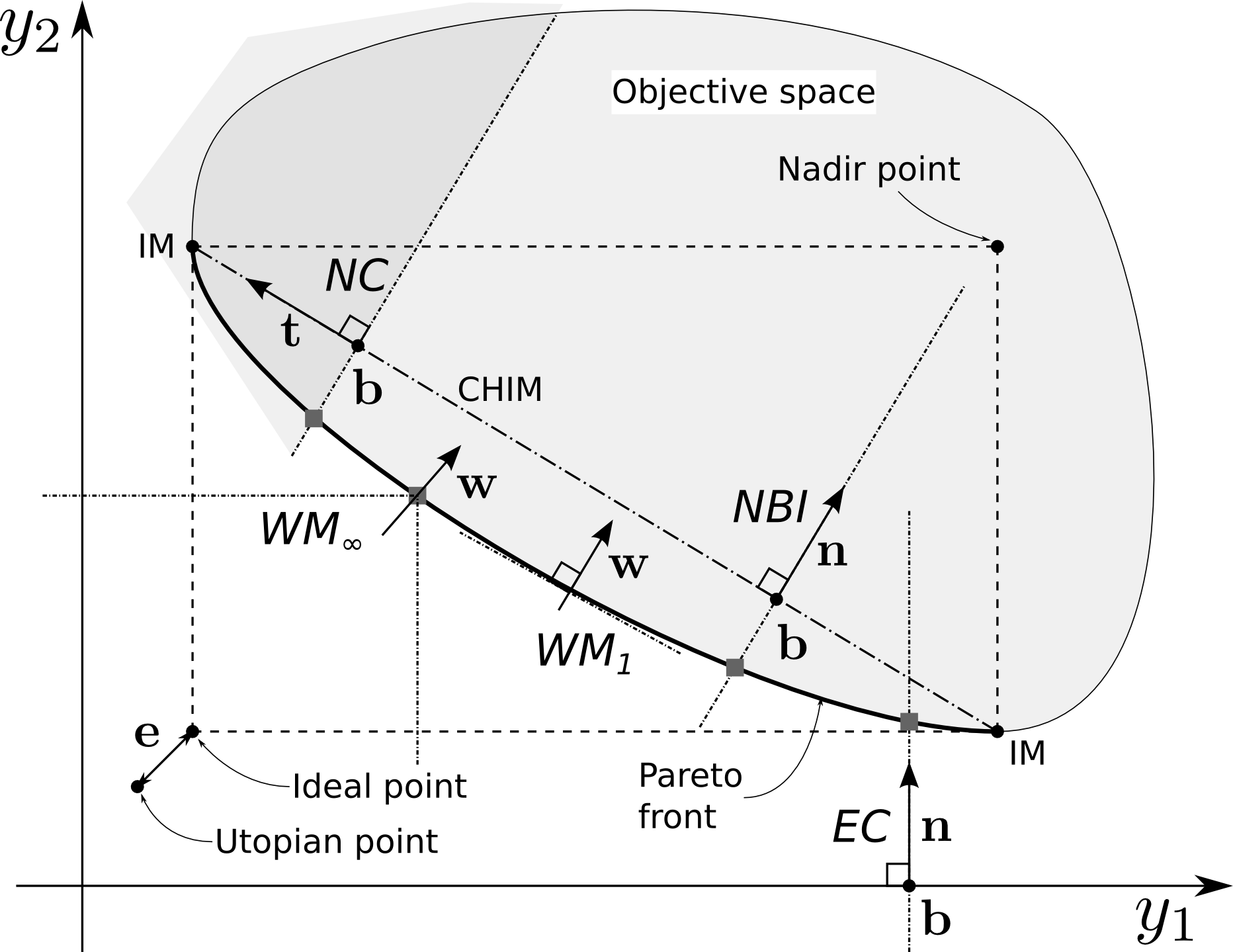
The weighted metric (WM) of ${\mathbf{f}}$ is defined as, $\displaystyle u_p({\mathbf{f}}) = \left(\sum_{i=1}^n w_i|f_i-f_i^{ref}|^p\right)^{1/p}$ where $p\in [1,\infty]$, $w_i>0$ and typically $\sum_{i=1}^n w_i=1$, and ${\mathbf{f}}^{ref}$ is a reference point.

The figure illustrates two special cases. The first one is $p=1$ ($WM_1$ in the figure), in which case the method is equivalent to the weighted sum method. This approach guarantees to find the complete Pareto front if it is convex. However, such is not guaranteed for non-convex case. Moreover, a uniform distribtuion of weights typically does not result in a uniformly distributed Pareto set. The second case is $p=\infty$ ($WM_\infty$ in the figure), where the method becomes the Tchebycheff metric. This approach guarantees to find the complete Pareto front no matter whether it is convex or not. However, the reference point has to satisfy ${\mathbf{f}}^{ref}\preceq{\mathbf{f}}^*$.

An extension of WM is the rotated WM, which will not be discussed in detail here.

A posteriori approach

The a posteriori approach is usually iterative and roughly fall into two categories. One is based on special formulations of mathematical programming, and can be considered an iterative a priori method that generates a Pareto point per iteration. The other, which is typically based on evolutionary algorithms (EAs), improves a set of (potential) Pareto points simultaneously per iteration.

Using mathematical programming

Two objectives

The two-objective problem has been studied extensively and is simpler than problems of more objectives. Two classical approaches are Normal Boundary Intersection (NBI) Das1998 and (Normalized) Normal Constraint (NC) Messac2003, as illustrated in the above figure. The NBI and NC can be considered the generalization of EC: Essentially, these methods convert the MO into an SO by introducing extra constraints and redefining the objective, so that the solution to the SO produces a point on the Pareto front. The extra constraints depends on a base point (or an anchor point) ${\mathbf{b}}$ on the CHIM, or the utopia line in two-objective case. A discrete approximation of the Pareto front is constructed by choosing various ${\mathbf{b}}$ along the utopia line and solving the resulting SO’s. As the reader might have noted, these approaches require the knowledge of the IM’s, which has to be solved before the application of the MO algorithms.

In the NBI formulation, the objective vector is constrained to be on a line defined by ${\mathbf{b}}$ and a direction vector ${\mathbf{n}}$ that is normal to the utopia line. The MO is converted to an SO for finding the intersection between the Pareto front and the line constraint, and hence the name NBI. $\displaystyle \begin{aligned} {\mathop{\mathrm{arg\,min}}\limits_{\mathbf{x}}} &\quad t({\mathbf{x}}) \\ {\mathrm{s.t.}}&\quad {\mathbf{x}}\in{\mathcal{X}}\\ &\quad {\mathbf{f}}={\mathbf{b}}+t{\mathbf{n}}\end{aligned}$

In the NC formulation, the objective is constrained to be on a half-plane defined by ${\mathbf{b}}$ and a direction vector ${\mathbf{t}}$ aligned with the utopia line. The MO is converted to an SO for finding the minimum of one of the objectives (the second objective in the illustrated case) given the extra constraint. $\displaystyle \begin{aligned} {\mathop{\mathrm{arg\,min}}\limits_{\mathbf{x}}} &\quad f_1({\mathbf{x}}) \\ {\mathrm{s.t.}}&\quad {\mathbf{x}}\in{\mathcal{X}}\\ &\quad ({\mathbf{f}}-{\mathbf{b}})\cdot{\mathbf{t}}\geq 0 \end{aligned}$ In [Messac2003], a normalization step is applied before solving the SO, which slightly simplifies the normal constraint.

Three or more objectives

The ideas of NBI and NC are easily extended to the cases of more objectives, as have been done in [Das1998] and [Messac2003]. However, both methods may not be able to explore the complete Pareto front, resulting in some unobtainable regions. This is illustrated in the figure below: Assuming the objective space is a sphere centered at the origin, the Pareto front ${\mathcal{F}}$ is an octant of the sphere (Green) and the CHIM is an equilateral triangle (Blue). However, the projection of the Pareto front on the CHIM plane, which is defined as CHIM+, is a region encompassed by three arcs (Red). That means, using a base point on the CHIM, one can only obtain solutions encompassed by the black dashed lines on the Pareto front.

As a remedy, Messac2004 proposed an improved NBI algorithm to explore the complete Pareto front by adding more base points outside the CHIM, i.e. on the CHIM+. Another approach, Directed Search Domain (DSD), is proposed in Erfani2011. In DSD, the NBI constraint is replaced by cone constraints that is able to explore the complete Pareto front by expanding or rotating the cone. The Messac2004 and Erfani2011 algorithms are more like patches to the classical NBI and NC algorithms. These “patched” algorithms contain empirical parameters that have to be tuned and there is no guarantee of finding the complete Pareto front.

More systematic algorithms are proposed in MG2009 as Successive Pareto Optimization (SPO) and in Motta2012 as Modified NBI and NC [Motta2012]. The two methods share a similar idea as recursive construction of the Pareto front. To solve an MO of $n$ objectives, i.e. find the $n$-dimensional Pareto front ${\mathcal{F}}$, $n$ problems of $n-1$ objectives are solved to generate the $n$ Pareto fronts $\partial{\mathcal{F}}$ of $(n-1)$ dimensions, which are the boundaries of ${\mathcal{F}}$. Subsequently, a set of base points are distributed uniformly between these boundaries, so as to cover the CHIM+ (almost) evenly and capture the complete Pareto front ${\mathcal{F}}$. Finally, at the recursion boundary, the SO’s associated with the objectives are solved to determine the IM’s.

Take a 3-objective problem for example, as shown in the figure below. First, the IM’s are found. Next, the NBI procedure is applied to find $\partial{\mathcal{F}}_{13}$ for the MO associated with objectives 1 and 3. Same procedures are done for $\partial{\mathcal{F}}_{12}$ and $\partial{\mathcal{F}}_{23}$. Finally, base points will be distributed over CHIM+, which is emcompassed by $\partial{\mathcal{F}}_{12}$, $\partial{\mathcal{F}}_{13}$ and $\partial{\mathcal{F}}_{23}$ ¹, to identify the complete Pareto front by applying the NBI procedure again.

Using evolutionary algorithm

There are two out-standing EAs in this category, which are Non-dominated Sorting Genetic Algorithm-II (NSGA-II) in Deb2002 and Strength Pareto Evolutionary Algorithm 2 (SPEA-2) in Zitzler2001. It appears they have become standard evolutionary algorithms for MO, against which new algorithms will be compared. However, I am not going to talk too much about EAs, which are not my favorite. Some introductory materials are found here. A comparison of evolutional algorithms for MO is found in, for example, Zitzler2000 and Bader2011.

Nevertheless, one important thing to learn from the EAs is the construction of the fitness function of a Pareto solution - How much it is dominating others, or how much it is improving the Pareto front? This requires the proper definition of indicators describing the quality of the Pareto front. These indicators have a broader range of application in, for example, the assessment of convergence and the construction of acquisition functions in Bayesian MO algorithms. In Zitzler2003, a number of criteria for the quality of the Pareto solution are gathered and compared. Three commonly used criteria include: The $\epsilon$, $R_2$ and hypervolume indicators.

The $\epsilon$-indicator characterizes the minimum separation between two Pareto solutions ${\mathcal{F}}$ and ${\mathcal{G}}$. The additive form is, $\displaystyle I_\epsilon({\mathcal{F}}, {\mathcal{G}}) = \inf_{\epsilon}\{\forall{\mathbf{g}}\in{\mathcal{G}}\exists{\mathbf{f}}\in{\mathcal{F}}: {\mathbf{f}}+\epsilon\preceq {\mathbf{g}}\}$ The multiplicative form is defined in a similar manner.

The $R_2$ indicator was initially developed in Hansen1998 for the case that the Pareto solutions are measured using a set of utility functions ${\mathcal{U}}$, e.g. the WM functions parameterized by the weight vectors ${\mathbf{w}}$. The utility fuctions are assigned some weights, or “probablities” $p(u)$, representing the preference information. The indicator is defined as the weighted or expected improvement of the best value of utility functions, $\displaystyle I_{R_2}({\mathcal{F}}, {\mathcal{G}}; {\mathcal{U}}) = \int_{u\in{\mathcal{U}}}[u^*({\mathcal{F}})-u^*({\mathcal{G}})]p(u)du$ where $u^*(\Box)=\inf\{ u({\mathbf{f}}),{\mathbf{f}}\in\Box \}$. When there is only one utility function, $I_{R_2}({\mathcal{F}},{\mathcal{G}})=u^*({\mathcal{F}})-u^*({\mathcal{G}})$.

The (binary) hypervolume indicator is defined as the “size” of the margin between two Pareto solutions ${\mathcal{F}}$ and ${\mathcal{G}}$, if one dominates the other. More formally, it is the measure $\Lambda$ of the set containing points that are dominated by ${\mathcal{F}}$ but not by ${\mathcal{G}}$, $\displaystyle I_H({\mathcal{F}}, {\mathcal{G}}) = \Lambda\{ {\mathbf{h}}|{\mathbf{h}}\succeq{\mathcal{F}}\wedge {\mathbf{h}}\preceq{\mathcal{G}}\}$

As mentioned above, there are two typical applications of these binary indicators. The first one is for convergence check. One can set one input to be the true Pareto solution (for benchmark problems), or a set consisting of the Utopian point (for real problems). The second application is to construct a unary indicator as the utility function of a potential solution ${\mathbf{f}}$ by setting ${\mathcal{F}}={\mathcal{G}}\cup\{ {\mathbf{f}}\}$, where ${\mathcal{G}}$ is a reference Pareto solution.

Bayesian MO algorithms

The algorithms to be discussed in this section are considered Bayesian because the optimization process generates the solution based on the observed samples of the objective functions, instead of the objective functions themselves as in classical methods. This bares the same idea as in the Bayesian SO algorithms. A surrogate has to be constructed using the observed samples as a replacement of the objective functions, or their utility function. During the optimization, the exploitation and exploration strategy has to be incorporated so as to account for the uncertainty of the surrogate model, as was done in Bayesian SO algorithms.

The Bayesian MO algorithms have deep roots in the classical methods. Depending on how classical methods are utilized, the algorithms are classified into the indirect and the direct methods.

Indirect methods

In the indirect methods, no special acquisition functions are developed for MO. Instead, the MO is converted to an SO as was done in the classical methods, such as WS and SPO. In a sense, the utility function in a classical method is directly used as an acqusition function. The resulting SO is solved using a BO algorithm, which is usually referred to as inner optimization.

One such example is the ParEGO algorithm in Knowles2006. This is probably the first important Bayesian MO algorithm. The utility function is developed using the augmented Tchebycheff function, which is a combination of the $u_\infty$ and $u_1$ functions, $\displaystyle u({\mathbf{f}}) = \max_i w_i f_i + \rho \sum_{i=1}^n w_i f_i$ where $\rho$ is a small positive value typically set to 0.05. In each run, a random weight vector is generated and a point on the Pareto front is found. A noteworthy disadvantage of ParEGO is that the uniformity of the Pareto solution is not guaranteed. Using a similar idea, the algorithms of EC, NBI, NC are easily combined with Bayesian SO algorithms.

A major disadvantage of the indirect method is that, in the inner optimization, the BO algorithm would cost multiple evaluations of the black-box objective functions only to find one point on the Pareto front. A more efficient approach would be the direct method, which produces one point on the Pareto front per evaluation.

Direct methods

In the direct methods, the BO algorithm is executed with special MO acquisition functions.

Two historical methods

One precursor in this category is Jeong2005. The MO is carried out using an evolutionary algorithm, where the fitness is defined as the expected improvements (EI) of the single objectives.

Another MO acquisition function is developed in Keane2006. It is the first paper extending EI and probablity of improvement (PoI) of SO to MO. The EI was defined as the product of the PoI and an Euclidean distance-based improvement function. However, the formulation is limited to the 2-objective case.

Two modern methods

Later, the concept of hypervolume is introduced into the development of MO acquisition functions. It is mainly developed into two families.

One family is the SMS-EGO method proposed in Ponweiser2008. It is an extension of the classical acqusition function of lower confidence bound (LCB), i.e. the improvement of HV due to LCB. In addition, a penalty is added to points that do not improve the Pareto front and an additive epsilon-dominance term is added to points close to Pareto front to smooth the distribution of the acquisition function. It was shown to outperform ParEGO and standard EAs like NSGA-II and SPEA-2. This method is easy to implement and has been widely used.

The other family is based on the S-metric expected improvement (SExI). It is the hypervolume version of EI for MO, originally proposed in Emmerich2005, as an extension of the classical EI for SO. The formulation is straight-forward by replacing the improvement function with the unary hypervolume indocator, $\displaystyle EI({\mathbf{x}}) = \int I({\mathbf{f}})p({\mathbf{f}};{\mathbf{x}})d{\mathbf{f}}$ where $I({\mathbf{f}}) = I_H({\mathcal{F}}\cup\{ {\mathbf{f}}\}, {\mathcal{F}})$ and ${\mathcal{F}}$ is the Pareto front of the current iteration.

In [Emmerich2005], the algorithm was called SMS-EMOA (i.e. solved using an evolutionary algorithm) and the integration of hypervolume was carried out using Monte Carlo method. In a later paper, Emmerich2008, an exact integration method is proposed for SExI. However, the computational complexity of the exact ingration method grows exponentially with the problem dimension and number of Pareto points.

The algorithm complexity of SExI definitely limits the spread of its application. There are even survey papers that skipped this algorithm in the numerical comparison section due to complexity in the implementation. Nevertheless, the SExI algorithm is improved in Hupkens2015, which claimed to be the fastest algorithm for the 2D and 3D cases. For the general case, however, the fastest algorithm is proposed in Couckuyt2014, which is based on the WFG algorithm. In [Couckuyt2014], the new algorithm is also applied to the MO version of PoI, which is easier to implement than SExI and appears to be equally effective.

Comparison

The aforementioned algorithms have been systematically compared in the literature. In Wagner2010, the algorithms from [Jeong2005], [Knowles2006], [Keane2006], [Ponweiser2008], and [Emmerich2008] are compared. Three necessary conditions are proposed to detect conceptual problems in the formulations while four desirable properties are identified. It is concluded that [Keane2006] is problematic. [Ponweiser2008] satisfies the essential conditions for acquisition function, but has disadvantages like non-smooth distribution of acquisition function. [Emmerich2008] has the most desirable properties, but is hard to implement.

In Zaefferer2013, four algorithms are compared: [Keane2006], [Emmerich2008], [Ponweiser2008], and an evolutional algorithm MSPOT (which I do not care), with SMS-EMOA as the baseline. [Keane2006] was found to be worse than the baseline, which agrees with the discussion in [Wagner2010]. The rest outperformed the baseline, but there was no decisive difference.

Further development

More algorithms and enhancements are developed in the literature since the proposal of SMS-EGO.

Multi-point proposal

With the advent of parallel computing, the idea of multi-point proposal was proposed, e.g. in Zhang2009. The idea is to find multiple candidate design vectors that improves the Pareto front and evaluate the black-box function at these new points simultaneously, exploiting the parallelism of the modern computers.

In Horn2015, algorithms like [Jeong2005], [Knowles2006] and [Ponweiser2008] are compared and extended with multi-point proposal. The major finding was that, for some algorithms, the multi-point variants did not significantly deteriorate the results. They even improved the approximation quality in some cases. Moreover, the change from the EI to the LCB could improve the results of the internal optimization within ParEGO.

Informatics-based approaches

This family of approaches are more recent and more “Bayesian” in the sense that a stronger statistical flavor is involved. Typical examples are stepwise uncertainty reduction (SUR) Picheny2015 and Predictive Entropy Search (PES) Hernández-Lobato2016. The idea is to pick a new point at each iteration to maximize the “information gain” to the current Pareto front. The information gain is typically measured using the Shannon entropy. These methods claim themselves to be “intuitive, statistically consistent and efficient”, as an alternative to the classical “sensible heuristic” approaches, such as the hypervolume EI. For academic problems, these methods do seem to be comparable to methods like SMS-EGO. However, the computational cost appears to be higher and the implementation seems to be more complex than all the methods discussed above.

Computer implementations

I have not found many implementations for Bayesian MO algorithms. Two working libraries I found are GPflowOpt and SUMO. There are some libraries for evolutionary MO algorithms, such as PyGMO and Platypus, but without surrogate capabilities. Probably these libraries can be incorporated into some BO framework for MO purposes.

Finally, for the evaluation of these libraries, there are a few standard test cases to play with:

1. MOP: VanVeldhuizen1999
2. ZDT: Zitzler2000
3. DTLZ: Deb2005