I am almost new to this field. Still learning.

Introduction

In the field of engineering, frequently we need to do system identification (SI), i.e. to infer the mathematical model of a dynamical system based on a set of time series data. A classical problem is the SI of a linear system ¹, $\displaystyle \begin{aligned} \dot{\mathbf{h}}&= {\mathbf{A}}{\mathbf{h}}+ {\mathbf{B}}{\mathbf{x}}\\ {\mathbf{y}}&= {\mathbf{C}}{\mathbf{h}}+ {\mathbf{D}}{\mathbf{x}}\end{aligned}$ Given input ${\mathbf{x}}$ and output ${\mathbf{y}}$, how does one determine the system matrices ${\mathbf{A}},{\mathbf{B}},{\mathbf{C}},{\mathbf{D}}$? Note that the system states ${\mathbf{h}}$ are not directly observed in the time series data, i.e. they are hidden. Over the long history of SI, many successful methods and algorithms have been developed. Some model the hidden states explicitly and some do not. Some can handle nonlinear systems and some do not. I am not an expert in SI and not going to talk about these algorithms.

In the machine learning community, it appears that people tend to reorganize and reformulate some old concepts into some “new ideas”. No offense. Indeed this is sometimes useful. In Hinton2013, several modeling methods for sequential data are divided into two categories: memoryless models and memoryful models. The memoryless models have limited memory window and the hidden state cannot be used efficiently. One example is the autoregressive model, which predicts the next term in a sequence from a fixed number of previous terms. Another example is the feed-forward neural nets, which generalize autoregressive models by using one or more layers of non-linear hidden units. The memoryful models infer the hidden state distribution at the cost of higher computational burden. One example is the linear systems algorithms that can be viewed as generative models with real-valued hidden states that cannot be observed directly. Another example is the hidden Markov models (HMM), which have a discrete one-of-N hidden state. In HMM, transitions between states are stochastic and controlled by a transition matrix. The outputs produced by a state are stochastic.

The last example of the memoryful models is the recurrent neural network (RNN), the topic of this post. It updates the hidden state in a deterministic nonlinear way. Compared to the aformentioned models, the RNN has the following advantages:

1. Distributed hidden state allows the efficient storage of information about the past.
2. Non-linear dynamics allows the update of hidden state in complicated ways.
3. No need to infer hidden state, whose evolution is purely deterministic.
4. Parameters in the RNN, i.e. the weights, are shared, which makes the model compact.

Mathematical Models of RNN

Vanilla RNN

This section is based on this.

The RNN centers around the following equation that describes the evolution of the hidden state, $\displaystyle {\mathbf{h}}_t = {\mathbf{f}}_W({\mathbf{h}}_{t-1}, {\mathbf{x}}_t)$ where ${\mathbf{f}}_W$ is an activation function with weights ${\mathbf{W}}$. The time steps $t$ and $t-1$ makes the formula recurrent. The function ${\mathbf{f}}_W$ and ${\mathbf{W}}$ may be shared between different layers/time steps.

A vanilla RNN is $\displaystyle \begin{aligned} {\mathbf{h}}_t &= \tanh({\mathbf{W}}_{hh} {\mathbf{h}}_{t-1} + {\mathbf{W}}_{xh} {\mathbf{x}}_t) \\ {\mathbf{y}}_t &= {\mathbf{W}}_{hy} {\mathbf{h}}_t \end{aligned}$ It looks very much like the linear system discussed above, except that it has a nonlinear state equation.

There are multiple types of RNNs: one-to-one, one-to-many, many-to-one, many-to-many, etc. In other words, the inputs ${\mathbf{x}}_t$ and outputs ${\mathbf{y}}_t$ are not necessarily nonzero. For example, an RNN is many-to-one when all of its inputs are assumed to be nonzero and only one output is expected (e.g. at the end) - this could be the case for a sequence classification problem.

Gradient Problem

There is an infamous issue with RNN: the gradient problem, which prevented the effective training of RNNs for a period of time.

The training of an RNN requires a proper definition of the error, or the scalar loss function $E$, $\displaystyle E = \sum_{t=1\ldots s} E_t({\mathbf{y}}_t, {\bar{\mathbf{y}}}_t)$ where $s$ time steps are assumed, and ${\bar{\mathbf{y}}}_t$ represent the ground truth.

The weights ${\mathbf{W}}$ are computed by the gradient descent method, where the gradient is computed from the back propagation (BP) of the error. In other words, one needs to obtain the derivative of $E$ w.r.t. ${\mathbf{W}}$ via the chain rule, $\displaystyle {\frac{\partial E}{\partial {\mathbf{W}}}} = \sum_{t=1,\ldots,s} {\frac{\partial E_t}{\partial {\mathbf{W}}}}$ where $\displaystyle {\frac{\partial E_t}{\partial {\mathbf{W}}}} = {\frac{\partial E_t}{\partial {\mathbf{y}}_t}} {\frac{\partial {\mathbf{y}}_t}{\partial {\mathbf{h}}_t}} {\frac{\partial {\mathbf{h}}_t}{\partial {\mathbf{W}}}}$

Now, focus on the weights for ${\mathbf{h}}$, i.e. ${\mathbf{W}}_{hh}$, which will be written as ${\mathbf{W}}$ for simplicity in the following. There is a “double dependency” in the gradient ${\frac{\partial {\mathbf{h}}_t}{\partial {\mathbf{W}}}}$: (1) ${\mathbf{h}}_t$ itself depends on all the past states; (2) a past state depends on the states prior to that state, too. Mathematically, $\displaystyle \begin{aligned} {\frac{\partial {\mathbf{h}}_t}{\partial {\mathbf{W}}}} &= \sum_{k=1,\ldots,t} {\frac{\partial {\mathbf{h}}_t}{\partial {\mathbf{h}}_k}} {\frac{\partial {\mathbf{h}}_k}{\partial {\mathbf{W}}}} \\ {\frac{\partial {\mathbf{h}}_t}{\partial {\mathbf{h}}_k}} &= \prod_{i=k+1,\ldots,t} {\frac{\partial {\mathbf{h}}_i}{\partial {\mathbf{h}}_{i-1}}} \end{aligned}$ where $\displaystyle {\frac{\partial {\mathbf{h}}_i}{\partial {\mathbf{h}}_{i-1}}} = \Lambda[{\mathbf{f}}_W']{\mathbf{W}}$ where $\Lambda$ makes the vector ${\mathbf{f}}_W'$ a diagonal matrix.

The gradient problem comes from the product in ${\frac{\partial {\mathbf{h}}_t}{\partial {\mathbf{h}}_k}}$. For each term of the product $\displaystyle \left\lVert {\frac{\partial {\mathbf{h}}_t}{\partial {\mathbf{h}}_k}} \right\rVert \le \lVert\Lambda[{\mathbf{f}}_W']\rVert \lVert {\mathbf{W}}\rVert \le \gamma_f \gamma_W$ where $\gamma_f$ and $\gamma_W$ are the maximum singular values of $\Lambda[{\mathbf{f}}_W']$ and ${\mathbf{W}}$, respectively. For the product $\displaystyle \left\lVert {\frac{\partial {\mathbf{h}}_t}{\partial {\mathbf{h}}_k}} \right\rVert \le (\gamma_f \gamma_W)^{t-k}$

When ${\mathbf{f}}_W$ is a function like $\tanh$, $\gamma_f$ would be close to zero as the input moves away from zero. As for ${\mathbf{W}}$, $\gamma_W$ is probably either $<1$ or $>1$. Therefore, a sufficiently large $t-k$, i.e. time span of dependency, can cause two issues for the BP,

1. Vanishing gradients: $\left\lVert {\frac{\partial {\mathbf{h}}_t}{\partial {\mathbf{h}}_k}} \right\rVert \rightarrow 0$, making ${\frac{\partial E_t}{\partial {\mathbf{W}}}}\sim 0$. In other words, the past states cannot be practically involved in BP.
2. Exploding gradients: $\left\lVert {\frac{\partial {\mathbf{h}}_t}{\partial {\mathbf{h}}_k}} \right\rVert \gg 1$, making ${\frac{\partial E_t}{\partial {\mathbf{W}}}}\gg 1$. In other words, the BP may experience a computational overflow.

Another way to see the gradient problem in the vanilla RNN is via the propagation of the variation/error of the hidden state ${\mathbf{h}}$. This way is somewhat hand-waving but more concise. The error of ${\mathbf{h}}_t$ is, $\displaystyle \delta {\mathbf{h}}_t = {\mathbf{f}}_W' \odot (\delta {\mathbf{W}}{\mathbf{h}}_{t-1} + {\mathbf{W}}\delta {\mathbf{h}}_{t-1})$ where $\odot$ is element-wise vector product and the variation associated with the input is ignored. The second term in the bracket represents the contribution of the error of the previous states to the error of the current state, $\displaystyle \delta {\mathbf{h}}_t \sim ({\mathbf{f}}_W'\odot {\mathbf{W}})^k \delta {\mathbf{h}}_{t-k}$ For situations discussed in the previous paragraph, the factor $({\mathbf{f}}_W'\odot {\mathbf{W}})^k$ can be (1) vanishing, so that $\delta{\mathbf{h}}_{t-k}$ almost does not contribute to $\delta{\mathbf{h}}_t$; (2) exploding, so that the contribution of $\delta{\mathbf{h}}_{t-k}$ overwhelms the contributions of the other states.

The issue of vanishing and exploding gradients does not mean the RNN model is impractical, but rather means that the gradient descent becomes increasingly inefficient when the temporal span of the dependencies increases.

There are some fixes to circumvent the gradient issue while retaining the vanilla RNN structure,

1. For vanishing gradients, one can perform a proper initialization of the weights, and incorporate a more well-behaved activation function, such as the rectified linear unit (ReLU): $f(x)=\max(0,x)$
2. For exploding gradient, one can do a clipping trick with a threshold $T$ for the gradient $\nabla$, $\displaystyle \nabla' = \frac{T}{\lVert\nabla\rVert^2}\nabla,\quad \mathrm{if}\quad \lVert\nabla\rVert^2 > T$

Long Short Term Memory

A more systematic solution to the vanishing gradient problem is the Long Short Term Memory (LSTM) model (Hochreiter1997) ². It introduces a “memory cell” that enables the storage and access of information over long periods of time. The state equation for LSTM is now significantly expanded from the vanilla RNN, $\displaystyle \begin{array}{rl} {\mathbf{i}}_t &= \sigma({\mathbf{W}}_{hi} {\mathbf{h}}_{t-1} + {\mathbf{W}}_{xi} {\mathbf{x}}_t + {\mathbf{b}}_i) \\ {\mathbf{f}}_t &= \sigma({\mathbf{W}}_{hf} {\mathbf{h}}_{t-1} + {\mathbf{W}}_{xf} {\mathbf{x}}_t + {\mathbf{b}}_f) \\ {\mathbf{o}}_t &= \sigma({\mathbf{W}}_{ho} {\mathbf{h}}_{t-1} + {\mathbf{W}}_{xo} {\mathbf{x}}_t + {\mathbf{b}}_o) \\ {\mathbf{g}}_t &= \tanh( {\mathbf{W}}_{hg} {\mathbf{h}}_{t-1} + {\mathbf{W}}_{xg} {\mathbf{x}}_t + {\mathbf{b}}_g) \\ {\mathbf{c}}_t &= {\mathbf{f}}_t \odot {\mathbf{c}}_{t-1} + {\mathbf{i}}_t \odot {\mathbf{g}}_t \\ {\mathbf{h}}_t &= {\mathbf{o}}_t \odot \tanh({\mathbf{c}}_t) \end{array}$ where $\sigma$ is the sigmoid function acting as a switch and ${\mathbf{b}}$ is a constant offset vector.

In the LSTM model, the current hidden state is no longer directly related to the current input and the previous hidden state. Rather, it is now an output from the memory cell ${\mathbf{c}}_t$. The memory cell is essentially a weighted sum of the past memory and the current information. In other words, it determines: (1) whether to activate the information from past steps, and (2) whether to overwrite the memory with the information from the current step. Specifically, three new gates are introduced,

1. Input gate: Scale input to cell (write)
2. Output gate: Scale output from cell (read)
3. Forget gate: Scale old cell values (reset)

The effect of the gates is better seen via the variation approach w.r.t. the hidden states, the memory cells, and the weights ${\mathbf{W}}_{hg}$. Note that ${\mathbf{W}}_{hg}$ corresponds to ${\mathbf{W}}_{hh}$ in the vanilla version and will again be written as ${\mathbf{W}}$ below for simplicity. Also note that, $\displaystyle \delta ({\mathbf{x}}\odot {\mathbf{y}}) = \delta {\mathbf{x}}\odot {\mathbf{y}}+ {\mathbf{x}}\odot \delta {\mathbf{y}}$

The variations of ${\mathbf{c}}_t$ and ${\mathbf{h}}_t$ are, $\displaystyle \begin{aligned} \delta {\mathbf{c}}_t &= {\mathbf{f}}_t\odot\delta {\mathbf{c}}_{t-1} + {\overline{\mathbf{W}}}\delta {\mathbf{h}}_{t-1} + {\mathbf{i}}_t\odot\delta {\mathbf{W}}{\mathbf{h}}_{t-1} \\ \delta {\mathbf{h}}_t &= \delta {\mathbf{o}}_t \odot \tanh({\mathbf{c}}_t) + {\mathbf{o}}_t \odot \tanh' \odot \delta {\mathbf{c}}_t \end{aligned}$ where ${\overline{\mathbf{W}}}$ is a condensed term containing several weights, including ${\mathbf{W}}_{hg}$. Note that ${\mathbf{W}}_{hg}$ only appears in the errors in the memory cell. Now, $\delta {\mathbf{h}}_t$ propagates into $\delta {\mathbf{c}}_t$ but $\delta {\mathbf{c}}_t$ does not necessarily propagate into ${\mathbf{h}}_{t-1}$. Instead, $\delta {\mathbf{c}}_t$ may be directly passed to $\delta {\mathbf{c}}_{t-1}$ without being affected by ${\mathbf{W}}_{hg}$, thus avoiding the products of ${\mathbf{W}}_{hg}$ and the gradient problems.

Gated Recurrent Unit

The gated recurrent unit (GRU) is another RNN variant Chung2015. It is similar to LSTM, but computationally more efficient, as there are less parameters and less complex structure.

Mathematically, GRU is represented as, $\displaystyle \begin{aligned} {\mathbf{r}}_t &= \sigma({\mathbf{W}}_{hr} {\mathbf{h}}_{t-1} + {\mathbf{W}}_{xr} {\mathbf{x}}_t + {\mathbf{b}}_r) \\ {\mathbf{u}}_t &= \sigma({\mathbf{W}}_{hz} {\mathbf{h}}_{t-1} + {\mathbf{W}}_{xz} {\mathbf{x}}_t + {\mathbf{b}}_z) \\ {\mathbf{g}}_t &= \tanh({\mathbf{W}}_{hg}({\mathbf{r}}_t\odot {\mathbf{h}}_{t-1}) + {\mathbf{W}}_{xg} {\mathbf{x}}_t + {\mathbf{b}}_g) \\ {\mathbf{h}}_t &= {\mathbf{u}}_t \odot {\mathbf{h}}_{t-1} + (1-{\mathbf{u}}_t) \odot {\mathbf{g}}_t \end{aligned}$

The GRU merges the cell state and hidden state, and thus ${\mathbf{h}}$ replaces ${\mathbf{c}}$ and the output gate ${\mathbf{o}}_t$ is no longer needed. Next, the GRU combines the forget and input gates into a single “update gate” ${\mathbf{u}}_t$, which enables the inclusion of long-term behaviors in the RNN. Finally, a reset gate ${\mathbf{r}}_t$ is added to control the contribution of the previous states to the current prediction.

While many alternative LSTM architectures have been proposed, in Greff2016, it was found that the original LSTM performs reasonably well on various datasets and none of the eight investigated modifications (including GRU) significantly improves performance. Furthermore, it was found that the forget gate and the output activation function as its most critical components.

Example

PyTorch: Windows with Anaconda

Among the popular machine learning frameworks, I chose PyTorch for its mild learning curve. I planed to try RNN on my Windows laptop, but it turns out PyTorch does not support Python 2 on Windows/Anaconda. So I did the following to install a minimal working PyTorch.

A Python 3 environment has to be created first by

1

conda create -n py36 python=3.6 anaconda

After a lengthy installation, the environment is then deployed by

1

conda activate py36

The command for installing PyTorch is found here. In my case where a GPU is not available, the PyTorch ecosystem is installed by,

1

conda install pytorch-cpu torchvision-cpu -c pytorch

The Python 3 installation might alter the default browser for the Jupyter Notebook. To reset the browser, first fo the following in the command line,

1

jupyter notebook --generate-config

And next specify the path to the browser in the config file,

1

c.NotebookApp.browser = u'path_to_browser %s'

Note that %s has to be in the string.

Toy Problem

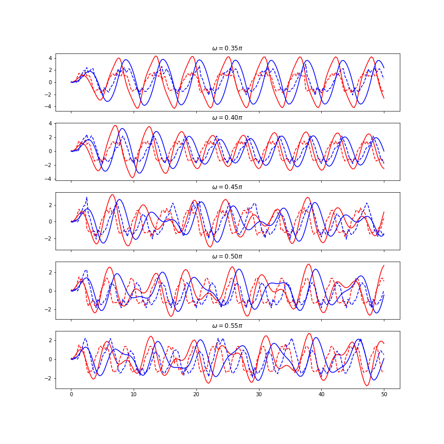
The dynamical system considered in this example is the forced Van der Pol (VdP) oscillator, $\displaystyle \ddot x = \mu (1-x^2) \dot x - x + A \sin(\omega t)$ where $\dot x$ and $x$ are considered the states of this second-order ODE. The first term on the RHS is a nonlinear damping term that introduced rich dynamical properties to the oscillator. The third term on the RHS is considered the input to the system. In this study, the following parameters are used, $\displaystyle \mu = 0.1,\quad A = 1.2,\quad x(0)=\dot x(0)=0,\quad t\in [0, 50],\quad \Delta t=0.25$ Given the sinusoidal input associated with a certain value of $\omega$, one can numerically integrate the system to obtain the response of the VdP oscillator. The goal of this exercise is to fit an RNN based on the VdP responses for several $\omega$’s, such that the RNN can reproduce the VdP responses for some other $\omega$’s.

The code implementation is adapted from here, and can be found from my github repo. Four types of RNNs are examined,

1. Vanilla RNN with $\tanh$ as activation function.
2. Vanilla RNN with ReLU as activation function.
3. LSTM RNN
4. GRU RNN

All the RNNs have one hidden layer with 32 states and one linear output layer. The RNNs are trained via the MSE loss function using the Adam algorithm with a learning rate of 0.01 and 10000 epochs. The training data set includes the VdP responses for $\omega=0.3\pi,0.4\pi,0.5\pi,0.6\pi$. The testing data sets includes the VdP responses for $\omega=0.35\pi,0.45\pi,0.55\pi$. In each training epoch, the data for gradient decent is a random segment (starts from beginning) of a VdP response randomly chosen from the training data set. A maximum of 120 time steps is used in the training. In other words, the last 80 time steps of the VdP response in the training data set are unseen by the RNN. Finally, the initial hidden states are set to be zero.

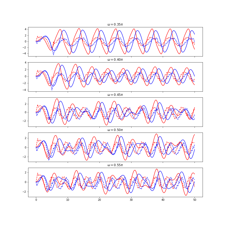
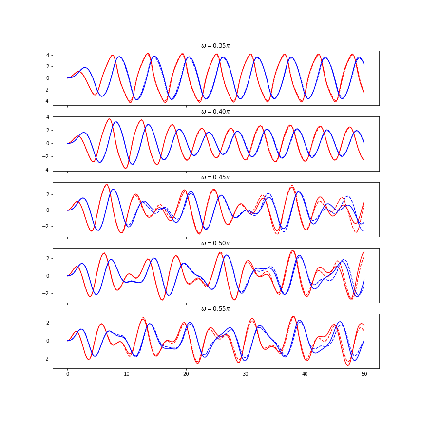
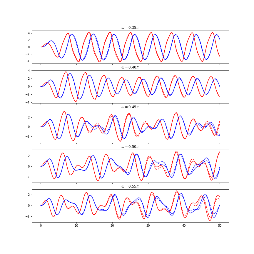
The results are shown in the figures below. The solid blue and red lines are the VdP responses found directly using numerical integration. The dashed lines are the RNN prediction. The vanilla RNNs do not do well in this problem. The failure probably can be explained the gradient vanishing problem that prevents the vanilla RNN to capture the long term periodic behavior. Both the LSTM and GRU do well. Note that the RNN predictions extrapolates well beyond the data used for training, as well as between the different values of $\omega$’s.

There are apprarently many tweaks and tunable parameters in the RNNs that can improve the prediction or generalize the model. For example,

1. What are the optimal numbers of layers and hidden states for the RNN?
2. What is the best way to utilize the training data set?
3. How to take care of different initial conditions? Maybe via infering the proper initial hidden state in RNN?
4. How to efficiently train the RNN for a larger parameter space that includes, e.g. $\mu, A, \omega$?

These might be done in a future post.

More References

1. Bengio et al, “Learning long-term dependencies with gradient descent is difficult”
2. Pascanu et al, “On the difficulty of training recurrent neural networks”
3. Recurrent Nets and LSTM
4. RNN Tutorial
5. Tips for training RNNs
6. Initial states for RNN